Unlocking Microbial Dark Matter: A Guide to High-Throughput Sequencing in Modern Ecology

Abstract

High-throughput sequencing (HTS) has revolutionized microbial ecology, moving research beyond mere cataloging to functional and mechanistic insights. This article provides researchers, scientists, and drug development professionals with a comprehensive overview of HTS technologies—from short-read Illumina to long-read PacBio and Oxford Nanopore platforms—and their applications in profiling complex microbiomes. It covers foundational concepts, methodological workflows, troubleshooting for optimization, and comparative validation of platforms, with a focus on leveraging these tools for biomedical discovery, therapeutic development, and understanding host-microbe interactions in health and disease.

The HTS Revolution: From Sanger Sequencing to Unraveling Complex Microbial Ecosystems

High-Throughput Sequencing (HTS), often referred to as Next-Generation Sequencing (NGS), represents a revolutionary technological advancement that has transformed genomics research by enabling the parallel sequencing of millions to billions of DNA fragments simultaneously [1] [2] [3]. This massive parallelization stands in stark contrast to traditional Sanger sequencing, which was limited by its minimal throughput and substantial cost [2] [4]. The core principle underlying all HTS technologies involves the fragmentation of DNA or RNA molecules into smaller pieces, followed by the attachment of adapters, parallel sequencing of these fragments, and subsequent computational reassembly of the sequences [2]. This fundamental approach has drastically reduced the time and cost associated with genomic studies while providing unprecedented scalability, making it possible to sequence entire genomes, transcriptomes, and epigenomes with remarkable speed and precision [2] [3].

The evolution of sequencing technologies has progressed through distinct generations, beginning with first-generation Sanger sequencing that enabled the landmark Human Genome Project but required 13 years and approximately $3 billion to complete [1]. The limitations of this method catalyzed the development of second-generation sequencing platforms (including Illumina and Ion Torrent) that dominated the HTS market for years, though they still relied on clonal amplification which could introduce bias and generated relatively short reads [1]. Most recently, third-generation sequencing technologies such as Pacific Biosciences (PacBio) Single Molecule, Real-Time (SMRT) sequencing and Oxford Nanopore Technology (ONT) have emerged, offering the ability to sequence single molecules without amplification and producing significantly longer reads [1] [3]. This technological progression has profoundly impacted microbial ecology research, allowing scientists to explore the vast complexity of microbial communities in environmental samples with unprecedented resolution [5] [6].

Key HTS Technology Platforms and Principles

Comparative Analysis of Major HTS Platforms

Table 1: Comparison of Major High-Throughput Sequencing Technologies

Technology	Sequencing Principle	Read Length	Accuracy	Throughput	Key Applications in Microbial Ecology
Illumina	Sequencing-by-synthesis with reversible dye terminators [1] [3]	Short to medium (150-300 bp) [1]	High [1] [2]	High [1]	16S rRNA amplicon sequencing, metagenomics, transcriptomics [7] [3]
Ion Torrent	Semiconductor sequencing detecting H+ ions [1] [3]	Short to medium (~200 bp) [1]	Moderate to high [1] [2]	Moderate to high [2]	Targeted amplicon sequencing, microbial genomics [2] [3]
PacBio SMRT	Single Molecule, Real-Time sequencing [1] [3]	Long (>10 kb) [1]	High (error rates <1%) [1]	Moderate [1]	De novo genome assembly, full-length 16S sequencing, epigenetic modification detection [1] [3]
Oxford Nanopore	Nanopore-based electrical signal detection [1] [3]	Long (>10 kb up to 4 Mb) [1]	Variable [1] [2]	Moderate to high [2]	Real-time pathogen surveillance, metagenome-assembled genomes, in-field sequencing [5] [2]

Detailed Technological Principles

Illumina Sequencing employs a sequencing-by-synthesis approach with reversible dye terminators [3]. The process begins with DNA fragmentation and adapter ligation, followed by bridge amplification on a glass slide that creates clusters of identical DNA fragments [1]. During sequencing cycles, fluorescently labeled nucleotides are incorporated, imaged, and then cleaved to allow the next incorporation cycle [1]. This method generates high-quality short-read data ideal for quantitative applications like transcriptomics and targeted sequencing [2].

Oxford Nanopore Technology operates on a fundamentally different principle by measuring changes in electrical current as DNA or RNA molecules pass through protein nanopores embedded in a membrane [1] [2]. The technology does not require amplification or fragmentation, enabling direct sequencing of native nucleic acids and providing ultra-long reads that are particularly valuable for assembling complete genomes from complex microbial communities [5] [2]. The portability of MiniON devices allows for real-time, in-field sequencing applications [2].

PacBio SMRT Sequencing utilizes zero-mode waveguides (ZMWs) - nanoscale wells that contain a single DNA polymerase molecule immobilized at the bottom [1]. As the polymerase incorporates fluorescently labeled nucleotides, the incorporation event is detected in real-time [1] [3]. This approach generates long reads with high accuracy, making it particularly suitable for resolving complex genomic regions and detecting epigenetic modifications in microbial genomes [1].

HTS Applications in Microbial Ecology

High-Throughput Sequencing has revolutionized microbial ecology by providing powerful tools to explore the immense diversity of microbial communities in environmental samples without the need for cultivation [5]. Metagenomics, enabled by HTS, allows researchers to recover metagenome-assembled genomes (MAGs) directly from environmental samples, dramatically expanding our knowledge of microbial diversity [5]. Recent studies utilizing long-read Nanopore sequencing of 154 complex soil and sediment samples successfully recovered 15,314 previously undescribed microbial species, expanding the phylogenetic diversity of the prokaryotic tree of life by 8% [5]. This demonstrates the remarkable power of HTS to uncover the vast, unexplored microbial dark matter.

Amplicon-based HTS approaches, such as 16S rRNA gene sequencing, have become standard for profiling microbial communities across diverse environments [7] [6]. These methods provide insights into microbial community structure, diversity, and dynamics in response to environmental changes and perturbations. For instance, HTS metabarcoding has been effectively employed to monitor the impact of agricultural practices on soil fungal communities, revealing how soil fumigation and biostimulant application alter microbial interactions and ecosystem functioning [7]. The technology has proven essential for understanding host-microbe interactions, biogeochemical cycling, and the ecological principles governing microbial community assembly and stability [6] [8].

Advanced applications in microbial ecology increasingly leverage the complementary strengths of multiple sequencing platforms. For example, the combination of short-read Illumina data for high accuracy and long-read Nanopore or PacBio data for improved genome assembly has enabled the recovery of high-quality microbial genomes from highly complex environments like soil [5]. Furthermore, the development of absolute quantification sequencing methods addresses the limitations of relative abundance data, providing more accurate characterization of microbial population dynamics and interactions [6].

Experimental Protocols for Microbial Ecology

Metagenome-Assembled Genome Recovery from Complex Soil Samples

Table 2: Essential Research Reagents and Materials for HTS in Microbial Ecology

Reagent/Material	Function	Application Example
DNA Extraction Kits	High-quality nucleic acid extraction from complex matrices	Soil, sediment, or water sample processing [5]
PCR Reagents	Amplification of target genes for amplicon sequencing	16S rRNA gene amplification for community profiling [7]
Sequence Adapters	Platform-specific ligation for library preparation	Illumina, Nanopore, or PacBio library construction [2]
Size Selection Beads	Fragment size selection for optimized sequencing	Magnetic bead-based clean-up and size selection [5]
Quality Control Kits	Assessment of DNA quality and quantity	Fluorometric quantification and fragment analysis [5]
Spike-in Standards	Absolute quantification of microbial abundances	Known quantity external standards for normalization [6]

The recovery of high-quality metagenome-assembled genomes from complex terrestrial habitats represents a grand challenge in metagenomics due to the enormous microbial diversity and complexity of these environments [5]. The following protocol outlines a robust workflow for MAG recovery using long-read sequencing:

Sample Collection and DNA Extraction:

• Collect soil or sediment samples using sterile corers and store immediately at -80°C to preserve nucleic acid integrity.
• Extract high-molecular-weight DNA using a protocol optimized for complex environmental samples, such as the CTAB-based method with subsequent purification.
• Assess DNA quality and quantity using fluorometry and pulsed-field gel electrophoresis to confirm high molecular weight.

Library Preparation and Sequencing:

• Prepare sequencing libraries without fragmentation to maintain long DNA molecules.
• For Nanopore sequencing: Use the ligation sequencing kit, paying particular attention to DNA repair and end-prep steps to maximize library complexity.
• Sequence with a PromethION flow cell, aiming for approximately 100 Gbp of data per sample to ensure sufficient coverage for genome reconstruction [5].

Bioinformatic Processing with mmlong2 Workflow:

• Perform metagenome assembly using Flye or similar long-read assemblers optimized for complex metagenomic data.
• Conduct iterative binning using multiple binners (e.g., MetaBAT2, MaxBin2) with differential coverage information from multiple samples.
• Apply the mmlong2 workflow, which includes ensemble binning and iterative refinement steps to improve MAG recovery from highly complex datasets [5].
• Assess MAG quality using CheckM or similar tools, retaining only medium and high-quality genomes based on completeness and contamination metrics.

Absolute Quantification Sequencing for Microbial Community Analysis

Traditional HTS approaches generate relative abundance data that can mask important population dynamics in microbial communities [6]. Absolute quantification sequencing addresses this limitation through the use of internal standards:

Spike-in Standard Preparation:

• Select or create DNA standards representing sequences not found in your sample type.
• Precisely quantify the standard using digital PCR or similar absolute quantification method.
• Add a known amount of spike-in standard to each sample prior to DNA extraction.

Library Preparation and Sequencing:

• Proceed with standard library preparation protocols appropriate for your sequencing platform.
• Include negative controls to assess background contamination.
• Sequence with sufficient depth to detect both rare community members and spike-in standards.

Data Analysis and Absolute Abundance Calculation:

• Process sequencing data through standard bioinformatic pipelines for amplicon or metagenomic analysis.
• Calculate absolute abundances using the formula: Absolute abundance = (Sample read count / Spike-in read count) × Known spike-in molecules.
• Analyze co-occurrence patterns and community assembly processes using absolute rather than relative abundances to avoid compositional data artifacts [6].

Technological Evolution and Future Perspectives

The evolution of HTS technologies has progressed remarkably from the first automated Sanger sequencers to the current landscape of diverse platforms each with unique strengths [4] [3]. Second-generation technologies dominated the market for over a decade, but recent advances in third-generation long-read sequencing are increasingly addressing their limitations regarding read length and amplification bias [1]. The continuing evolution of HTS is characterized by several key trends: the convergence of long-read and short-read technologies to leverage their complementary advantages, the development of more sophisticated bioinformatic tools to handle increasingly complex datasets, and the emergence of novel applications that push the boundaries of what can be achieved with sequencing technologies [5] [3].

Future developments in HTS will likely focus on enhancing the accuracy and sensitivity of sequencing data, reducing costs further, improving the accessibility of the technology, and developing more efficient and scalable computational solutions for data analysis [3]. For microbial ecology specifically, the integration of absolute quantification methods, multi-omics approaches, and synthetic microbial ecosystem studies will provide unprecedented insights into the principles governing microbial community assembly, stability, and function [6] [8]. As these technologies continue to evolve and become more accessible, they will undoubtedly uncover new dimensions of microbial diversity and function, further expanding our understanding of the microbial world and its critical roles in ecosystem health and functioning.

The landscape of high-throughput sequencing for microbial ecology is dominated by three major platforms: Illumina, Pacific Biosciences (PacBio), and Oxford Nanopore Technologies (ONT). Each employs a distinct sequencing biochemistry, leading to complementary strengths in output, resolution, and application.

Illumina technology utilizes sequencing-by-synthesis with reversible dye-terminators. This approach generates massive volumes of short reads (typically 300-600 bp for MiSeq/NovaSeq systems) with very high per-base accuracy (Q30, >99.9%). For 16S rRNA gene sequencing, it typically targets specific hypervariable regions (e.g., V3-V4, ~450 bp) [9] [10]. This high accuracy makes it a benchmark for quantitative abundance measurements.

PacBio employs Single Molecule, Real-Time (SMRT) sequencing. DNA polymerase incorporates fluorescently tagged nucleotides into a template immobilized at the bottom of a zero-mode waveguide. Its key innovation is Circular Consensus Sequencing (CCS), where a single DNA molecule is sequenced repeatedly in a loop. This produces long, accurate reads known as HiFi reads, which combine long read lengths (10-25 kb) with high accuracy (Q27, ~99.9%) [9] [11]. This is ideal for sequencing the full-length 16S rRNA gene (~1,500 bp).

Oxford Nanopore Technologies (ONT) is based on the passage of single DNA or RNA strands through protein nanopores embedded in an electrical-resistant membrane. Each nucleotide base causes a characteristic disruption in the ionic current as it passes through the pore, enabling real-time, long-read sequencing. Early versions had higher error rates, but recent chemistries (R10.4.1 flow cells) and basecalling algorithms have significantly improved accuracy to over 99% [9] [12] [10]. ONT can sequence full-length 16S rRNA amplicons and is notable for its portability and real-time data stream.

Table 1: Technical Comparison of Sequencing Platforms for 16S rRNA Amplicon Sequencing

Feature	Illumina	PacBio HiFi	Oxford Nanopore
Sequencing Chemistry	Sequencing-by-synthesis	SMRT (Single Molecule, Real-Time)	Nanopore-based electronic sensing
Typical 16S Read Length	Short (300-600 bp, e.g., V3-V4)	Long (Full-length, ~1,450 bp)	Long (Full-length, ~1,400-1,500 bp)
Key Read Type	Short reads	HiFi (High-Fidelity) reads	Continuous long reads
Per-base Accuracy	Very High (~Q30, >99.9%)	Very High (~Q27, ~99.9%)	Moderate-High (Recent: >Q20, >99%) [9] [12]
Primary 16S Application	Amplicon (hypervariable regions)	Full-length 16S rRNA gene sequencing	Full-length 16S rRNA gene sequencing
Typical Output per Run	High (Millions of reads)	Moderate	Variable (Scalable from MinION to PromethION)
Run Time	1-3 days	0.5-2 days	1-72 hours (real-time) [10]
Species-Level Resolution	Lower (e.g., 48% in rabbit gut) [9]	Higher (e.g., 63% in rabbit gut) [9]	Highest (e.g., 76% in rabbit gut) [9]

Performance in Microbial Ecology Studies

Comparative studies reveal how these platform characteristics translate into performance for profiling complex microbial communities, such as those found in the gut, soil, and respiratory tract.

Taxonomic Resolution

A key advantage of long-read sequencing is improved taxonomic resolution. A 2025 study on rabbit gut microbiota directly compared the three platforms, demonstrating a clear hierarchy in species-level classification rates: ONT (76%), followed by PacBio (63%), and then Illumina (48%) [9]. Full-length 16S rRNA sequences allow for analysis across all nine hypervariable regions, providing more phylogenetic information for discriminating between closely related species than single or paired hypervariable regions [12] [10].

However, a significant challenge across all platforms is the high proportion of sequences assigned to "uncultured_bacterium" at the species level, highlighting limitations in current reference databases rather than the technologies themselves [9].

Diversity Metrics and Community Composition

The choice of platform can influence the observed microbial community structure:

• Alpha Diversity (Richness/Evenness): Illumina often captures greater species richness, likely due to its higher sequencing depth and accuracy, which can better detect rare taxa. Community evenness, however, is often comparable between platforms [10].
• Beta Diversity (Between-Sample Differences): Studies show that while overall community patterns are consistent, the specific platform and primer choice can create a significant "batch effect" in beta diversity analyses. For instance, a rabbit gut study found significant differences in taxonomic composition between Illumina, PacBio, and ONT, even after using standardized bioinformatics [9]. This effect can be more pronounced in complex microbiomes like soil or gut compared to lower-biomass environments like the respiratory tract [10].
• Taxonomic Abundance Biases: Platform-specific biases in taxonomic abundance are well-documented. For example, a respiratory microbiome study using the ANCOM-BC2 tool found that ONT overrepresented certain taxa like Enterococcus and Klebsiella while underrepresenting others like Prevotella and Bacteroides compared to Illumina [10]. These biases may stem from differences in DNA extraction, PCR amplification, or the sequencing chemistry itself.

Table 2: Comparative Performance in Microbial Community Analysis

Performance Metric	Illumina	PacBio HiFi	Oxford Nanopore
Species-Level Classification Rate	Lower (e.g., 48%) [9]	Medium (e.g., 63%) [9]	Higher (e.g., 76%) [9]
Detection of Rare Taxa	Excellent (High depth)	Good	Good, but can be influenced by error rate
Quantitative Accuracy (Abundance)	High (Gold standard)	High	Good, with modern error-correction
Bias in Taxonomic Profile	Under-represents GC-rich regions [13]	More uniform genome coverage	Can over/under-represent specific taxa [10]
Community Differentiation	Clear clustering by sample type [12]	Clear clustering by sample type [12]	Clear clustering by sample type, but may show platform-specific separation [9] [12]

Detailed Experimental Protocols

Below are standardized protocols for 16S rRNA amplicon sequencing on each platform, as applied in recent microbial ecology studies.

Illumina 16S rRNA (V3-V4) Amplicon Sequencing Protocol

This protocol is adapted from the Illumina 16S Metagenomic Sequencing Library Preparation guide and used in recent comparative studies [9] [10].

• Step 1: PCR Amplification. Amplify the target hypervariable region (e.g., V3-V4) from genomic DNA using region-specific primers (e.g., S-D-Bact-0341-b-S-17 / S-D-Bact-0785-a-A-21) [9]. A typical reaction uses 2X KAPA HiFi HotStart ReadyMix and the following cycling conditions: 95°C for 3 min; 25 cycles of 95°C for 30 s, 55°C for 30 s, 72°C for 30 s; final extension at 72°C for 5 min.
• Step 2: Library Indexing and Amplification. A second, limited-cycle PCR reaction (8 cycles) is performed to attach dual indices and sequencing adapters using the Nextera XT Index Kit.
• Step 3: Library Pooling and Clean-up. The indexed PCR products are purified using magnetic beads (e.g., AMPure XP), quantified, and normalized. Libraries are then pooled in equimolar amounts.
• Step 4: Sequencing. The pooled library is denatured, diluted, and loaded onto an Illumina flow cell (e.g., MiSeq Reagent Kit v3) for paired-end sequencing (e.g., 2 × 300 cycles).

PacBio Full-Length 16S rRNA Amplicon Sequencing Protocol

This protocol leverages PacBio's HiFi read capability for highly accurate full-length 16S sequences [9] [12].

• Step 1: Full-Length 16S Amplification. Amplify the full-length 16S rRNA gene (~1,500 bp) from genomic DNA using universal primers (e.g., 27F and 1492R), which are tailed with PacBio barcode sequences for multiplexing. A typical reaction uses KAPA HiFi HotStart DNA Polymerase and the following cycling conditions: 95°C for 2 min; 27-30 cycles of 98°C for 20 s, 57°C for 30 s, 72°C for 60 s; final extension at 72°C for 5 min [9].
• Step 2: Library Preparation. The amplified and barcoded DNA is pooled in equimolar concentrations. A SMRTbell library is constructed using the SMRTbell Express Template Prep Kit 2.0 or 3.0, which involves DNA repair, A-tailing, and adapter ligation to create the circularizable template [9] [12].
• Step 3: Sequencing on Sequel II/IIe System. The prepared library is bound to polymerase, loaded onto a SMRT Cell, and sequenced on a Sequel II or IIe system using a Sequel II Binding Kit and Sequencing Kit. The run is configured for CCS mode to generate HiFi reads.

Oxford Nanopore Full-Length 16S rRNA Amplicon Sequencing Protocol

This protocol is based on the ONT Microbial Amplicon Barcoding Kit (SQK-MAB114.24), which offers a rapid and flexible workflow [14] [15].

• Step 1: Full-Length 16S or ITS Amplification. Amplify the target gene using the provided 16S or ITS primers (e.g., 27F and 1492R) and a high-fidelity master mix (e.g., LongAmp Hot Start Taq 2X Master Mix). Cycling conditions: 95°C for 1 min; 35-40 cycles of 95°C for 20 s, 58°C for 30 s, 65°C for 2 min; final extension at 65°C for 5 min [14].
• Step 2: Amplicon Barcoding (Rapid Adapter Ligation). The PCR amplicons are directly barcoded using the kit's Amplicon Barcodes 01-24 in a rapid, 15-minute reaction that simultaneously inactivates the barcodes [14].
• Step 3: Sample Pooling and Clean-up. The barcoded samples are pooled and purified using AMPure XP beads to remove short fragments and reagents [14].
• Step 4: Adapter Ligation and Loading. The Rapid Adapter is ligated to the purified, barcoded amplicons in a 5-minute reaction. The library is then immediately primed and loaded onto a MinION flow cell (R10.4.1 recommended) for sequencing [14] [10].

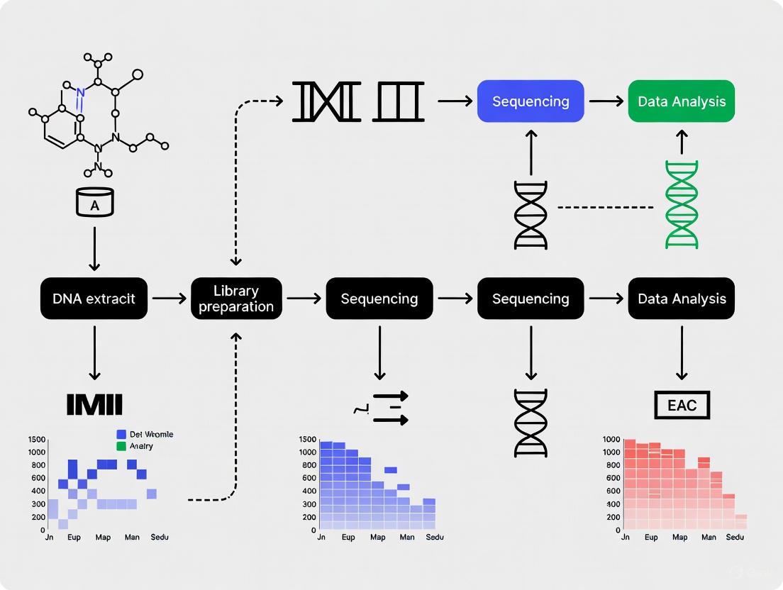
Diagram 1: 16S rRNA Sequencing Workflow Comparison. The workflow diverges during library preparation, where platform-specific primers and chemistries are applied, then reconverges for downstream bioinformatic analysis.

Research Reagent Solutions and Essential Materials

Table 3: Essential Reagents and Kits for 16S rRNA Amplicon Sequencing

Item	Function/Description	Example Products / Kits
gDNA Extraction Kit	Isolates high-quality, inhibitor-free genomic DNA from complex samples (feces, soil, sputum).	Quick-DNA Fecal/Soil Microbe Microprep Kit (Zymo Research) [12], DNeasy PowerSoil Kit (QIAGEN) [9]
PCR Enzyme Master Mix	Amplifies the target 16S rRNA region with high fidelity and yield.	KAPA HiFi HotStart ReadyMix (Roche), LongAmp Hot Start Taq 2X Master Mix (NEB) [14]
Library Prep Kit (Illumina)	Prepares amplicons for sequencing on Illumina systems, including indexing.	16S Metagenomic Sequencing Library Prep Protocol [9], QIAseq 16S/ITS Region Panel (Qiagen) [10]
Library Prep Kit (PacBio)	Creates SMRTbell libraries from amplicons for HiFi sequencing.	SMRTbell Express Template Prep Kit 2.0/3.0 (PacBio) [9] [12]
Library Prep Kit (ONT)	Rapid barcoding and adapter ligation for nanopore sequencing.	Microbial Amplicon Barcoding Kit 24 V14 (SQK-MAB114.24) (ONT) [14] [15]
Magnetic Beads	Size selection and clean-up of PCR products and final libraries.	AMPure XP Beads (Beckman Coulter) [9] [14]
Flow Cell	The consumable where sequencing occurs.	MiSeq Reagent Kit (Illumina), SMRT Cell (PacBio), MinION Flow Cell (R10.4.1) (ONT) [14] [10]
Quality Control Tools	Quantifies and qualifies DNA and libraries pre-sequencing.	Qubit Fluorometer & dsDNA HS Assay (Thermo Fisher) [9], Fragment Analyzer (Agilent) [9]

Application Notes and Implementation Guidance

Platform Selection Guide

Choosing the optimal platform depends on the specific research objectives, budget, and infrastructure [10]:

• Choose Illumina MiSeq/NextSeq when: The primary goal is high-throughput, cost-effective profiling of microbial communities at the genus level. It is ideal for large-scale cohort studies where high accuracy and depth are critical for detecting rare taxa and quantifying abundances [9] [10].
• Choose PacBio Revio/Sequel IIe when: The research demands high-resolution, species-level taxonomy from amplicons and requires the highest possible accuracy for long reads. It is the preferred choice for generating publication-quality, full-length 16S data where budget is less constrained [9] [11] [12].
• Choose ONT MinION/PromethION when: The application requires species-level resolution, real-time data stream, portability for in-field sequencing, or the flexibility to run a few to many samples on demand. Its rapid workflow enables same-day results [15] [10].

Critical Considerations for Experimental Design

• Database Limitations: A significant bottleneck is not the technology but reference databases. A high proportion of species-level assignments may be labeled "uncultured_bacterium," limiting biological insights [9]. Curated, environment-specific databases can improve annotation.
• Primer and Platform Effects: The combination of primer choice and sequencing platform can introduce significant biases in perceived community composition. It is strongly discouraged to directly compare or merge datasets generated with different platforms or primer sets without appropriate batch-effect correction [9].
• Bioinformatic Pipelines: The optimal data processing pipeline differs by platform. Illumina and PacBio HiFi data are typically processed with DADA2 for Amplicon Sequence Variants (ASVs), while ONT data may require specialized tools like the EPI2ME 16S workflow, Emu, or Spaghetti to handle its unique error profile [9] [10].

Within the framework of high-throughput sequencing for microbial ecology research, selecting the appropriate method for microbiome analysis is a critical first step that fundamentally shapes the scope and validity of a study's findings. The two predominant methodologies—amplicon sequencing and shotgun metagenomics—offer distinct lenses through which to examine microbial communities [16]. Amplicon sequencing, which involves the targeted amplification and sequencing of conserved marker genes like the 16S rRNA gene for bacteria and archaea, has been a cornerstone of microbial ecology for decades, providing a cost-effective means of assessing taxonomic composition [17] [18]. In contrast, shotgun metagenomics employs an untargeted approach, randomly sequencing all DNA fragments within a sample to simultaneously reveal taxonomic identity and functional potential [19] [20]. The choice between these techniques is not a matter of superiority but of alignment with the specific research question, considering factors such as required taxonomic resolution, the need for functional insight, sample type, and available resources [16] [21]. This application note provides a structured comparison of these platforms and details standardized protocols to guide researchers in making an informed selection and generating high-quality data for their investigations in microbial ecology and drug development.

Comparative Analysis: Amplicon Sequencing vs. Shotgun Metagenomics

A direct comparison of the technical and practical aspects of amplicon and shotgun sequencing reveals a clear trade-off between resource expenditure and informational yield. The decision matrix must balance the research objectives against practical constraints.

Table 1: Core Methodological Comparison between Amplicon and Shotgun Metagenomic Sequencing

Feature	Amplicon Sequencing	Shotgun Metagenomics
Principle	Targeted amplification of specific marker genes (e.g., 16S, 18S, ITS) [17]	Untargeted, random sequencing of all DNA in a sample [20]
Typical Taxonomic Resolution	Genus-level; sometimes species-level, highly dependent on region targeted [21] [22]	Species-level and often strain-level; enables detection of single nucleotide variants [21]
Functional Profiling	Not available directly; possible only via prediction algorithms (e.g., PICRUSt) [21]	Yes, provides direct insight into functional gene content and metabolic pathways [19] [20]
Organisms Detected	Primarily bacteria & archaea (16S); fungi (ITS); microbial eukaryotes (18S) [17]	All domains: bacteria, archaea, eukaryotes, and viruses [20] [21]
Cost per Sample	Lower; cost-effective for large-scale studies [17] [18]	Higher; typically 2-3x the cost of amplicon sequencing [21]
Bioinformatic Complexity	Moderate; well-established, standardized pipelines (e.g., QIIME 2, DADA2) [20] [22]	High; requires sophisticated resources and tools for assembly, binning, and annotation [20] [22]
Host DNA Contamination	Low risk due to targeted amplification [21]	High risk; can dominate sequencing data, requiring depletion strategies or deep sequencing [21]
Primary Applications	Phylogenetic studies, biodiversity assessments, microbial composition analysis across large sample cohorts [17] [18]	Functional potential analysis, pathogen discovery, strain-level tracking, genome reconstruction (MAGs) [19] [20]

Table 2: Quantitative and Performance Metrics Based on Empirical Data

Metric	Amplicon Sequencing	Shotgun Metagenomics
Sensitivity in Low-Biomass Samples	High; due to PCR amplification of target [18]	Lower; unless subjected to deep sequencing, which increases cost [20]
Correlation with Biomass	Variable; can be skewed by primer mismatches and gene copy number variation [16]	Stronger; generally provides a better correlation between read abundance and biomass [16]
Data Sparsity	Higher; detects only a fraction of the community revealed by shotgun [22]	Lower; captures a broader and more even community profile [22]
Alpha Diversity	Lower reported values compared to shotgun [22]	Higher reported values; captures greater microbial richness [22]
Database Dependency	Relies on 16S/ITS databases (e.g., SILVA, Greengenes) [22]	Relies on whole-genome databases (e.g., NCBI RefSeq, GTDB) [22]

Experimental Protocols

Protocol 1: 16S rRNA Amplicon Sequencing for Bacterial Profiling

This protocol outlines a standardized method for characterizing bacterial communities via amplification and sequencing of the 16S rRNA gene hypervariable regions, optimized for the Illumina MiSeq platform.

3.1.1 Sample Preparation and DNA Extraction

• Sample Collection: Preserve samples immediately after collection. For stool, skin, or environmental samples, use sterile, DNA-free containers and flash-freeze in liquid nitrogen or store at -80°C. For stabilization without freezing, use nucleic acid preservation buffers like RNAlater [19].
• DNA Extraction: Extract high-molecular-weight DNA using kits designed for complex samples (e.g., DNeasy PowerLyzer PowerSoil Kit (Qiagen) or NucleoSpin Soil Kit (Macherey-Nagel)) [22]. Include negative extraction controls to monitor reagent contamination. Quantify DNA using fluorometric methods (e.g., Qubit) to ensure accurate normalization.

3.1.2 Library Preparation and Sequencing

• PCR Amplification: Amplify the hypervariable V3-V4 region using primers 341F (5'-CCTACGGGNGGCWGCAG-3') and 805R (5'-GACTACHVGGGTATCTAATCC-3') [22].
  • Reaction Mix: 2x KAPA HiFi HotStart ReadyMix, 10 μM each primer, and 10-50 ng template DNA.
  • Cycling Conditions: 95°C for 3 min; 25-30 cycles of 95°C for 30 s, 55°C for 30 s, 72°C for 30 s; final extension at 72°C for 5 min [22].
• Amplicon Clean-up: Purify PCR products using magnetic beads (e.g., AMPure XP) to remove primers and dimers.
• Indexing PCR & Pooling: Add dual indices and Illumina sequencing adapters in a second, limited-cycle PCR. Quantify amplicons, normalize equimolarly, and pool into a single library.
• Sequencing: Sequence on an Illumina MiSeq with v3 chemistry, targeting 50,000 paired-end reads per sample to achieve saturation in diversity curves [18].

3.1.3 Bioinformatic Analysis Pipeline

• Demultiplexing: Assign raw sequencing reads to samples based on their unique barcodes.
• Quality Filtering & Trimming: Use DADA2 (v1.22+) to filter reads based on quality profiles, trim primers, and truncate reads (e.g., 290 bp forward, 230 bp reverse) [22].
• Inference of ASVs: Apply the DADA2 algorithm to learn error rates and infer amplicon sequence variants (ASVs), providing single-nucleotide resolution.
• Taxonomic Assignment: Classify ASVs against the SILVA (v138) or Greengenes2 reference database. For enhanced species-level classification, a complementary k-mer-based classification with Kraken2/Bracken2 against the NCBI RefSeq database is recommended [22].
• Data Export: Generate a feature table (ASVs), a taxonomy table, and a phylogenetic tree for downstream ecological analysis.

Protocol 2: Shotgun Metagenomic Sequencing for Comprehensive Community Analysis

This protocol details a workflow for shotgun metagenomics, enabling simultaneous taxonomic profiling at high resolution and functional characterization of microbial communities.

3.2.1 Sample Preparation and DNA Extraction

• High-Quality DNA Extraction: The foundation of a successful shotgun library is high-molecular-weight, high-purity DNA. Use kits validated for metagenomics (e.g., NucleoSpin Soil Kit) [22]. For samples with high host DNA contamination (e.g., tissue, blood), implement host DNA depletion kits (e.g., NEBNext Microbiome DNA Enrichment Kit) to increase microbial sequence yield [21].
• DNA QC: Assess DNA integrity via agarose gel electrophoresis or Fragment Analyzer and quantify via fluorometry.

3.2.2 Library Preparation and Sequencing

• Library Construction: Fragment 100-500 ng of input DNA via acoustic shearing (Covaris) to a target size of 350-550 bp. Use a commercial library prep kit (e.g., Illumina DNA Prep) for end-repair, A-tailing, and adapter ligation [20]. Perform limited-cycle PCR to index libraries.
• Library QC and Pooling: Quantify final libraries by qPCR and confirm size distribution using a Bioanalyzer. Pool libraries equimolarly.
• Sequencing: Sequence on an Illumina NovaSeq 6000 to a depth of 20-50 million paired-end (2x150 bp) reads per sample for complex communities like gut microbiota or soil [21] [22]. Deeper sequencing (e.g., 100+ million reads) may be required for metagenome-assembled genome (MAG) reconstruction.

3.2.3 Bioinformatic Analysis Pipeline

• Pre-processing: Remove adapter sequences and low-quality bases using Trimmomatic or fastp.
• Host Read Removal: Align reads to the host genome (e.g., GRCh38 for human-associated samples) using Bowtie2 and discard matching reads [22].
• Taxonomic Profiling: Directly classify reads against a curated genome database (e.g., Unified Human Gastrointestinal Genome (UHGG) database or GTDB) using tools like Kraken2 and quantify abundances with Bracken [22].
• Functional Profiling: Align reads to a functional database (e.g., KEGG, eggNOG) using HUMAnN3 to determine pathway abundances [21].
• De Novo Assembly and Binning: For MAG recovery, assemble quality-filtered reads into contigs using metaSPAdes. Bin contigs into draft genomes using metaBAT2. Check MAG quality (completeness, contamination) with CheckM [19].

The Scientist's Toolkit: Essential Research Reagents and Materials

Table 3: Key Research Reagent Solutions for Metagenomic Workflows

Item	Function/Application	Example Products/Kits
DNA Extraction Kit	Isolation of high-quality, high-molecular-weight DNA from complex samples.	NucleoSpin Soil Kit (Macherey-Nagel), DNeasy PowerLyzer PowerSoil Kit (Qiagen) [22]
Host DNA Depletion Kit	Selective removal of host genomic DNA from samples with high host:microbe ratio.	NEBNext Microbiome DNA Enrichment Kit [21]
16S rRNA PCR Primers	Amplification of specific hypervariable regions for amplicon sequencing.	341F/805R for V3-V4 region [22]
Library Preparation Kit	Preparation of sequencing-ready libraries from fragmented DNA.	Illumina DNA Prep Kit [20]
DNA Quantitation Kits	Accurate quantification of DNA and final library concentrations.	Qubit dsDNA HS Assay Kit
Bioinformatics Tools	For data processing, analysis, and interpretation.	QIIME 2, DADA2 (Amplicon) [22]; Kraken2, HUMAnN3, metaSPAdes, metaBAT2 (Shotgun) [19] [22]
Reference Databases	For taxonomic classification and functional annotation.	SILVA, Greengenes (16S) [22]; UHGG, GTDB, KEGG (Shotgun) [22]
KHKI-01215	KHKI-01215, MF:C24H26F3IN6O, MW:598.4 g/mol	Chemical Reagent
m-PEG26-NHS ester	m-PEG26-NHS ester, MF:C58H111NO30, MW:1302.5 g/mol	Chemical Reagent

The strategic choice between amplicon and shotgun metagenomics is pivotal for the success of any microbial ecology research project. Amplicon sequencing remains a powerful, cost-efficient tool for large-scale studies focused on compositional differences and broad taxonomic profiling, particularly in well-defined systems or when sample biomass is low [18] [21]. Conversely, shotgun metagenomics is the unequivocal choice for studies demanding high taxonomic resolution, comprehensive functional insight, or genome-level reconstruction, despite its higher computational and financial costs [19] [20]. As the field advances, the integration of both methods—using amplicon sequencing for broad screening and shotgun on a subset for in-depth analysis—or the harmonization of datasets from both platforms presents a powerful approach to leverage their respective strengths [23]. By aligning the methodological choice with the core research question and adhering to the robust protocols outlined herein, researchers can effectively harness the power of high-throughput sequencing to unravel the complexities of microbial ecosystems.

The field of microbial ecology has been revolutionized by culture-independent methods that allow the identification and characterization of microorganisms from all domains of life directly from their environment [24]. Two primary methodological approaches have emerged as cornerstones of modern microbiome research: marker gene sequencing (primarily targeting the 16S rRNA gene) and whole-genome shotgun (WGS) metagenomics [24]. The development of these approaches, coupled with advanced high-throughput sequencing technologies, has enabled researchers to move beyond cataloging microbial membership to understanding functional capabilities and ecological dynamics within complex microbial communities [24].

Marker gene studies provide a targeted analysis of specific taxonomic groups by sequencing conserved genetic regions, while WGS metagenomics sequences the total DNA content of a sample, enabling comprehensive profiling of biodiversity and functional potential [24]. The choice between these techniques depends on the research questions, with each offering distinct advantages and limitations that must be considered in experimental design. These technological advances have opened new frontiers in understanding microbial communities' roles in human health, environmental processes, and biotechnological applications.

Methodological Foundations

16S rRNA Gene Sequencing

The 16S ribosomal RNA gene is a cornerstone of microbial ecology, serving as a phylogenetic marker for identifying and classifying bacteria and archaea. This approach leverages conserved regions for primer binding and variable regions for taxonomic differentiation [25].

Key Workflow Steps:

• DNA Extraction and Target Amplification: Microbial DNA is extracted from samples, and the 16S rRNA gene (or specific variable regions like V3-V4) is amplified using universal primers.
• Library Preparation and Sequencing: Amplified products are prepared into sequencing libraries compatible with platforms such as Illumina MiSeq.
• Bioinformatic Processing: Raw sequences are quality-filtered, denoised into Amplicon Sequence Variants (ASVs), and classified against reference databases.

Table: Common 16S rRNA Hypervariable Regions and Their Applications

Region	Length (bp)	Taxonomic Resolution	Common Applications
V1-V3	~500	Genus to species	Broad-range bacterial diversity
V3-V4	~450	Genus-level [25]	Human gut microbiome studies [25]
V4	~250	Genus-level	Environmental samples, high-throughput studies
Full-length 16S	~1500	Species-level [25]	High-resolution taxonomic profiling

Advanced Protocol: Species-Level Identification with V3-V4 Regions

Traditional analysis of the V3-V4 regions is often limited to genus-level classification. However, a novel pipeline achieves species-level identification by addressing the limitation of fixed similarity thresholds [25].

Experimental Protocol:

• Database Construction:

  • Integrate seed sequences from authoritative databases (SILVA, NCBI RefSeq, LPSN) [25].
  • Supplement with 16S rRNA sequences from 1,082 human gut samples to improve coverage, particularly for anaerobes and uncultured organisms [25].
  • Create a non-redundant ASV database specific to the V3-V4 regions (positions 341–806) [25].

• Threshold Determination:

  • Establish flexible, species-specific classification thresholds (ranging from 80% to 100%) instead of a fixed 98.5% cutoff [25].
  • Define precise thresholds for 896 common human gut species to resolve misclassification between closely related species [25].

• Taxonomic Classification with ASVtax Pipeline:

  • Apply dynamic thresholds for accurate taxonomic classification of new ASVs [25].
  • Combine k-mer feature extraction, phylogenetic tree topology, and probabilistic models for precise annotation [25].

This methodology significantly enhances species-level classification from V3-V4 data, facilitating more reliable ecological and functional interpretations [25].

Whole-Genome Shotgun Metagenomics

WGS metagenomics sequences the total DNA from a sample without targeting specific genes, enabling functional profiling and the reconstruction of metagenome-assembled genomes (MAGs) [24].

Key Workflow Steps:

• DNA Extraction and Library Preparation: Extract total genomic DNA, with optional host DNA depletion for low-biomass samples. Prepare sequencing libraries without PCR amplification where possible.
• High-Throughput Sequencing: Sequence using Illumina (short-read) or PacBio/Oxford Nanopore (long-read) platforms.
• Bioinformatic Analysis: Quality control, assembly, binning into MAGs, and taxonomic/functional annotation.

Table: Comparison of Sequencing Technologies for Metagenomics

Technology	Read Length	Throughput	Key Advantages	Limitations
Illumina	150-300 bp	Up to 6 Tb (NovaSeq) [24]	High accuracy, low cost per base	Short reads complicate assembly
PacBio HiFi	10-25 kb	1-6 Tb (DNBSEQ-T7) [24]	Long, accurate reads ideal for MAGs [26]	Higher cost, more DNA required
Oxford Nanopore	Up to hundreds of kb	~10 Gb per run (MinION) [24]	Ultra-long reads, real-time analysis	Higher error rate (~2.5%) [24]

Advanced Protocol: Genome-Resolved Metagenomics with Long Reads

Long-read sequencing technologies are overcoming the "grand challenge" of recovering high-quality genomes from highly complex environments like soil [5]. The following protocol is adapted from the mmlong2 workflow used to recover over 15,000 previously undescribed microbial species from terrestrial habitats [5].

Experimental Protocol:

• Deep Long-Read Sequencing:

  • Perform deep sequencing of environmental samples (e.g., ~100 Gbp per sample using Nanopore) to ensure sufficient coverage of rare taxa [5].
  • Target a median read N50 of >6 kbp to facilitate assembly across repetitive regions [5].

• Metagenome Assembly and Processing:

  • Assemble reads into contigs using long-read assemblers (e.g., Canu, Flye).
  • Polish assemblies with original read data to improve accuracy.
  • Remove eukaryotic contigs based on taxonomic classification.

• Iterative Binning with MMLong2:

  • Circular MAG Extraction: Identify and extract circular contigs as separate genome bins [5].
  • Differential Coverage Binning: Incorporate read mapping information from multi-sample datasets to leverage abundance variations across samples [5].
  • Ensemble Binning: Apply multiple binning algorithms (e.g., MetaBAT2, MaxBin2) to the same metagenome and consolidate results [5].
  • Iterative Binning: Repeat the binning process on the unbinned contigs from the initial round to recover additional MAGs [5].

• Quality Assessment and Dereplication:

  • Assess MAG quality (completeness, contamination) using CheckM or similar tools.
  • Dereplicate MAGs at species level (e.g., 95% average nucleotide identity) to create a non-redundant genome catalogue [5].

This protocol enables cost-effective recovery of high-quality microbial genomes from highly complex ecosystems, which remain an untapped source of biodiversity [5].

Data Analysis and Integration

Microbial Community Analysis

Alpha Diversity Analysis

Alpha diversity metrics describe species richness, evenness, or diversity within a single sample [27]. They are grouped into four complementary categories, each capturing different aspects of microbial communities [27].

Table: Essential Alpha Diversity Metrics for Microbiome Studies

Category	Key Metrics	Biological Interpretation	Notes
Richness	Chao1, ACE, Observed ASVs	Estimates the total number of species (observed and unobserved)	Highly correlated with each other; Chao1 and ACE account for unobserved species [27].
Dominance/Evenness	Berger-Parker, Simpson, ENSPIE	Measures the dominance of a few microbes over others	Berger-Parker is easily interpretable (proportion of the most abundant taxon) [27].
Phylogenetic Diversity	Faith's PD	Incorporates evolutionary relationships between species	Depends on both the number of observed features and singletons [27].
Information Theory	Shannon, Pielou's evenness	Combines richness and evenness based on entropy	All information metrics are strongly correlated as they use Shannon's entropy as a reference [27].

Practical Recommendations [27]:

• Report a comprehensive set of metrics from at least three categories (e.g., Observed ASVs, Berger-Parker, Faith's PD, Shannon) to capture different diversity aspects.
• Do not rely solely on rarefaction; calculate metrics with non-rarefied data to preserve information, but validate with rarefied datasets.
• Note that singletons (ASVs with only one read) are required for some metrics (e.g., Robbins), but are removed by DADA2.

Statistical Comparisons Between Communities

Comparing microbial communities requires specialized statistical approaches. The ∫-LIBSHUFF program calculates the integral form of the Cramér-von Mises statistic to determine whether differences in library composition are due to sampling artifacts or underlying biological differences [28].

Application Protocol:

• Input: A distance matrix generated by DNADIST (PHYLIP package) containing distances for comparisons between two or more 16S rRNA gene libraries [28].
• Method: The algorithm measures the number of sequences unique to one library when two libraries are compared across all phylogenetic levels [28].
• Interpretation: Small P-values for both comparisons (X vs. Y and Y vs. X) indicate strong evidence that neither library is a subset of the other, suggesting distinct communities [28].

Data Integration Strategies

Integrating microbiome data with other omics layers, such as metabolomics, is crucial for elucidating complex biological mechanisms. A comprehensive benchmark of nineteen integrative methods provides the following guidelines [29].

Table: Strategies for Integrating Microbiome and Metabolome Data

Research Goal	Recommended Methods	Application Notes
Global Associations	MMiRKAT, Mantel test	Determine the presence of an overall association between entire microbiome and metabolome datasets [29].
Data Summarization	Redundancy Analysis (RDA), MOFA2	Identify major trends and sources of variability that are shared across the two omic layers [29].
Individual Associations	Sparse PLS (sPLS), Spearman correlation with multiple testing correction	Detect specific microbe-metabolite pairs that are significantly associated [29].
Feature Selection	sparse CCA (sCCA), LASSO	Identify a minimal set of the most relevant microbial and metabolic features that drive the association [29].

Essential Preprocessing Considerations [29]:

• Compositionality: Properly handle microbiome compositionality using transformations like centered log-ratio (CLR) or isometric log-ratio (ILR).
• Data Structures: Account for over-dispersion, zero-inflation, and high collinearity inherent in microbiome data.
• Study Design: Control for confounders such as transit time, regional changes, and horizontal transmission in the study design and analysis.

Experimental Planning and Visualization

The Scientist's Toolkit: Research Reagent Solutions

Table: Essential Materials for Microbiome Studies

Reagent/Material	Function	Application Notes
ZymoBIOMICS DNA Kit	Standardized microbial DNA extraction	Ensize reproducible lysis of Gram-positive and negative bacteria
PBS Buffer	Sample dilution and homogenization	Maintains cellular integrity during processing
MagAttract PowerSoil DNA Kit	High-throughput DNA extraction	Ideal for soil and sediment samples with high inhibitor content
Illumina MiSeq Reagent Kits	16S rRNA amplicon sequencing	Standardized workflow for V3-V4 or V4 regions
PacBio SMRTbell Libraries	HiFi shotgun metagenomics	Enables long-read sequencing with high accuracy [26]
MetaPolyzyme Enzyme Mix	Mechanical and enzymatic lysis	Enhances DNA yield from difficult-to-lyse microorganisms
RNAlater Stabilization Solution	Sample preservation	Stabilizes microbial community composition at time of collection
Yo-Pro-3	Yo-Pro-3, MF:C26H31I2N3O, MW:655.4 g/mol	Chemical Reagent
Linoleyl myristate	Linoleyl myristate, MF:C32H60O2, MW:476.8 g/mol	Chemical Reagent

Workflow Visualization

The following diagram illustrates the integrated workflow for 16S rRNA and whole-genome shotgun metagenomics, highlighting their complementary nature in microbial ecology studies.

Data Visualization Guidelines

Effective visualization is crucial for interpreting highly dimensional, sparse, and compositional microbiome data [30].

Table: Selection Guide for Microbiome Data Visualization

Analysis Type	Sample-Level Plot	Group-Level Plot	Key Considerations
Alpha Diversity	Scatterplot	Box plot with jitters	Show individual data points to visualize distribution [30].
Beta Diversity	Dendrogram, Heatmap	PCoA ordination plot	Use PCoA for overall variation between groups; dendrograms for sample relationships [30].
Relative Abundance	Heatmap	Stacked bar chart, Pie chart	Aggregate rare taxa in bar charts to avoid overcrowding [30].
Core Taxa	-	UpSet plot	Use UpSet plots instead of Venn diagrams for >3 groups [30].
Microbial Interactions	Network plot	Correlogram	Highlight key associations and modular structure [30].

Optimization Tips [30]:

• Colors: Use consistent, color-blind friendly palettes (e.g., viridis) across all figures. Limit to 7 colors per graph.
• Labels: Add informative titles and axis labels. Label outliers or key features, but avoid overplotting.
• Ordering: Reorder categories by median, abundance, or user-defined order rather than alphabetically.
• Faceting: Split complex graphs into panels (e.g., by phylum) to improve readability.

The integration of 16S rRNA sequencing and whole-genome shotgun metagenomics provides a powerful framework for advancing microbial ecology research. While 16S rRNA profiling offers a cost-effective method for taxonomic profiling and diversity analyses, WGS metagenomics enables functional insights and genome-resolved metagenomics through MAG recovery [24]. The emergence of long-read sequencing technologies addresses previous limitations in studying complex environments, substantially expanding known microbial diversity and improving species-level classification [25] [5]. As these technologies continue to evolve, standardized workflows, appropriate statistical integration methods, and effective visualization practices will be essential for translating microbial ecology data into meaningful biological insights with applications in human health, environmental science, and biotechnology.

High-throughput sequencing (HTS) technologies have revolutionized microbial ecology by enabling comprehensive study of microbial communities directly from their environments, bypassing the limitation that most environmental microbes cannot be cultivated in the laboratory [31] [32]. These culture-independent approaches, particularly shotgun metagenomic and metatranscriptomic sequencing, allow researchers to simultaneously characterize taxonomic composition and functional potential of complex microbial ecosystems [31] [33]. The synergy between HTS, powerful computing hardware, and sophisticated bioinformatics software has transformed our understanding of microbial diversity, ecological interactions, evolutionary histories, and community metabolism [32]. This protocol outlines essential bioinformatics methodologies for processing sequencing data from raw reads through taxonomic classification and functional analysis, framed within the context of investigating microbial ecology using HTS technologies.

Metagenomic analyses generally follow two complementary approaches: read-based classification (useful when organisms have close relatives in reference databases) and assembly-based analysis (preferable for exotic environments with poorly represented organisms) [34]. A typical integrated workflow incorporates elements of both strategies to maximize insights into microbial community structure and function.

Table 1: Key Analysis Approaches in Metagenomics

Approach	Description	Best Use Cases	Common Tools
Read-Based Classification	Direct taxonomic and functional assignment of individual sequencing reads	Samples with good reference database representation; quick community profiling	Kaiju, DIAMOND, Kraken, MetaPhlAn [31] [34]
Assembly-Based Analysis	Reconstruction of genomic sequences from short reads before analysis	Discovering novel organisms; studying genomic context	MEGAHIT, SPAdes, IDBA-UD, MetaVelvet-SL [31] [34]
Binning	Grouping contigs or reads into biologically meaningful units	Reconstructing genomes from complex communities	CONCOCT, metaBAT, MaxBin [31]
Single-Cell Genomics	Sequencing genomes from individually isolated cells	Studying rare community members; reference genome creation	Single-cell genomic sequencing [31]

Metagenomic Analysis Workflow: This diagram illustrates the two primary analysis pathways (read-based and assembly-based) for processing microbial sequencing data, from raw reads through to biological interpretation.

Materials and Reagents

Table 2: Key Research Reagent Solutions for Metagenomic Analysis

Category	Tool/Resource	Primary Function	Application Context
Quality Control	fastp [34]	Adaptive read trimming and quality reporting	Preprocessing of raw sequencing data
Taxonomic Classification	Kaiju [33] [34]	Protein-based taxonomic assignment using translated reads	Sensitive taxonomy profiling
Alignment	DIAMOND [34]	Fast protein sequence alignment	Functional annotation against reference databases
Assembly	MEGAHIT [34]	Efficient metagenome assembly	Contig reconstruction from short reads
Workflow Management	Snakemake [33] [34]	Workflow automation and reproducibility	Pipeline execution and management
Reference Databases	NCBI nr [33]	Non-redundant protein sequence database	Taxonomic and functional reference
Reference Databases	Gene Ontology (GO) [33]	Functional term standardization	Functional annotation consistency

Step-by-Step Protocol

Data Preprocessing and Quality Control

Objective: Remove low-quality sequences and contaminants to ensure reliable downstream analysis.

Procedure:

• Quality Assessment: Run fastp on raw FASTQ files to generate quality reports. Examine key metrics including per-base sequence quality, sequence duplication levels, and adapter contamination [34].
• Read Trimming: Execute quality and adapter trimming with fastp using parameters: --cut_front --cut_tail --cut_window_size 4 --cut_mean_quality 20 [34].
• Host DNA Depletion: (Optional) For host-associated samples, align reads to host genome using Bowtie2 with sensitive parameters. Retain unmapped reads for subsequent analysis [33] [34].
• Post-processing QC: Verify trimming effectiveness by comparing pre- and post-trimming quality reports.

Technical Notes: The fastp tool processes input reads in a single pass, generating interactive HTML reports that include before-and-after filtering statistics [34].

Taxonomic Profiling Methods

Objective: Identify microbial community composition at various taxonomic ranks.

Reference-Based Taxonomic Classification

Procedure:

• Database Selection: Choose appropriate reference database based on sample type (e.g., Greengenes for 16S rRNA gene studies, NCBI nr for shotgun data) [31].
• Classification Execution: Run Kaiju using the -t parameter to specify taxonomy nodes and -f for reference database. For standard metagenomes: kaiju -t nodes.dmp -f nr_euk.fmi -i sample1.fastq -o sample1.kaiju.out [33] [34].
• Result Processing: Convert Kaiju outputs to abundance tables using Kaiju2table script, applying abundance filters (recommended: 0.001% cutoff) to remove likely false positives [33].
• Cross-Tool Validation: (Optional) Run complementary classification with MetaPhlAn or Kraken for method verification [31].

Reference-Free Operational Taxonomic Unit (OTU) Analysis

Procedure:

• Gene Targeting: For amplicon studies, select appropriate marker genes (16S rRNA for general composition; RuBisCO, amoA, soxB, mcrA for specific biogeochemical cycles) [31].
• Sequence Clustering: Use UCLUST or UPARSE to cluster sequences into OTUs at 97% similarity threshold [31].
• Chimera Removal: Apply UCHIME or ChimeraSlayer to filter artificial chimeras formed during PCR amplification [31].
• Taxonomic Assignment: Assign taxonomy to representative sequences using RDP classifier or PhylOTU for phylogenetic placement of unclassified OTUs [31].

Technical Notes: Protein-based classification with Kaiju generally provides greater sensitivity for species-level identification compared to 16S rRNA-based methods, particularly for poorly characterized organisms [33].

Functional Annotation

Objective: Characterize metabolic potential and functional processes within microbial communities.

Procedure:

• Protein Identification: Align quality-filtered reads to NCBI nr database using DIAMOND with sensitive mode: diamond blastx -d nr -q sample1_trimmed.fastq -o sample1.daa -f 100 --sensitive [34].
• Gene Ontology Mapping: Transfer functional annotations using custom SQLite database that maps protein accessions to GO terms [33].
• Abundance Quantification: Generate normalized counts for each GO term by summing proportional read counts across all proteins associated with each term [33].
• Functional Profile Analysis: Create sample-by-function abundance matrices for comparative analysis between experimental conditions.

Technical Notes: MetaFunc constructs a specialized SQLite database that consolidates GO annotations from all identical sequences in NCBI nr entries, ensuring comprehensive functional annotation coverage [33].

Metagenome Assembly and Binning

Objective: Reconstruct genomes from complex microbial communities without reference sequences.

Procedure:

• De Novo Assembly: Execute MEGAHIT with meta-large preset for complex communities: megahit -1 sample1_R1.fastq -2 sample1_R2.fastq -o assembly_output --preset meta-large [34].
• Assembly Quality Assessment: Evaluate contig statistics (N50, contig counts) and check for chimeric sequences using appropriate validation tools [31].
• Sequence Binning: Group contigs into genome bins using composition-based tools (CONCOCT, metaBAT) with tetra-nucleotide frequency and coverage information [31].
• Bin Refinement: Integrate multiple binning approaches and use CheckM to assess genome completeness and contamination.

Technical Notes: Composition-based binning methods are computationally intensive but can be accelerated using matrix decomposition approaches like streaming singular value decomposition [31].

Integrated Multi-Omics Analysis: This workflow illustrates the parallel processing of microbial and host-derived sequences in metatranscriptomic studies, enabling correlation analysis between host gene expression and microbial community function.

Data Analysis and Interpretation

Statistical Analysis of Community Composition

Objective: Identify differentially abundant taxa and functions between experimental conditions.

Procedure:

• Data Normalization: Filter low-abundance features using filterbyExpr function in edgeR with minimum count threshold of 1 (user-adjustable) [33].
• Normalization Factor Calculation: Compute normalization factors using calcNormFactors in edgeR with default TMM (Trimmed Mean of M-values) method [33].
• Differential Analysis: Perform exact tests for pairwise comparisons between experimental groups using exactTest in edgeR [33].
• Multiple Testing Correction: Apply Benjamini-Hochberg false discovery rate (FDR) correction to p-values [33].
• Result Interpretation: Consider both statistical significance (FDR < 0.05) and biological relevance (fold-change > 2) when identifying important features.

Correlation Analysis Between Taxonomy and Function

Objective: Establish relationships between microbial taxa and functional processes.

Procedure:

• Data Integration: Merge taxonomic abundance tables with functional annotation tables using taxonomy IDs and protein accession numbers as keys [33].
• Correlation Calculation: Compute Spearman correlation coefficients between taxon abundances and functional term abundances.
• Network Visualization: Create bipartite networks linking taxa to functions using Cytoscape or specialized R packages.
• Biological Interpretation: Identify keystone taxa driving important metabolic processes and potential functional redundancies within communities.

Troubleshooting and Optimization

Table 3: Common Bioinformatics Challenges and Solutions

Problem	Potential Causes	Solutions
Low taxonomic classification rate	Reference database bias; novel organisms	Enrich with environmental sequences; use assembly-based approach [31]
Chimeric contigs in assembly	Misassembly of similar regions from different genomes	Apply composition-based binning; use coverage variation across samples [31]
Inconsistent functional annotations	Different reference databases or identifier systems	Use standardized mapping dictionaries; create custom SQLite databases [33] [34]
High computational demands	Large dataset size; memory-intensive algorithms	Use disk-based aligners (DIAMOND); implement streaming algorithms [31] [34]
Difficulty discriminating closely related species	Highly conserved marker genes	Combine multiple marker genes; use protein-level classification [31] [33]

Applications in Microbial Ecology

The protocols described enable diverse applications in microbial ecology research. The STAMP (Sequence Tag-based Analysis of Microbial Populations) method, which utilizes genetically barcoded organisms, can quantify population bottlenecks and founding population sizes during infection, revealing host barriers to colonization and microbial dissemination patterns [35]. For human microbiome studies, the integration of host transcriptomic data with microbial functional profiling enables investigation of host-microbe interactions in conditions like colorectal cancer [33]. In environmental microbiology, these approaches help uncover the roles of microbial communities in biogeochemical cycling, symbiosis, and responses to environmental change [31] [32].

The bioinformatics workflows presented here provide a comprehensive framework for analyzing metagenomic and metatranscriptomic sequencing data, from raw reads through taxonomic and functional interpretation. As sequencing technologies continue to advance, bioinformatics methods must similarly evolve to address new computational challenges and leverage the richer data structures provided by long-read sequencing and chromatin conformation capture technologies [31]. The integration of standardized, reproducible workflows like MEDUSA [34] and MetaFunc [33] with continuously updated reference databases will further enhance our ability to extract meaningful biological insights from complex microbial communities, ultimately advancing our understanding of microbial ecology in diverse environments from the human body to global ecosystems.

From Sample to Insight: Practical HTS Workflows and Cutting-Edge Applications

Within microbial ecology research, high-throughput sequencing has revolutionized our capacity to decipher complex microbial communities. The reliability of these insights, however, is fundamentally dependent on the wet-lab protocols employed for DNA extraction and library preparation [36]. These initial steps are critical for determining the quantity, quality, and representativeness of the sequenced data, ultimately influencing all downstream ecological inferences. This application note provides detailed methodologies for key experiments, summarizing comparative data and outlining essential research reagents to support robust experimental design in microbial ecology.

Experimental Protocols

DNA Extraction Methods for Challenging Samples

The recovery of DNA from complex biological samples, particularly those that are ancient or environmentally challenging, requires specialized protocols optimized for short, fragmented DNA and the removal of co-extracted inhibitors [36].

Protocol 1: QG Extraction Method (Rohland and Hofreiter, 2007) This silica-based method is designed for efficient DNA release and inhibitor removal [36].

• Digestion: Incubate the biological sample (e.g., 50-100 mg of dental calculus or soil) in a digestion buffer containing EDTA and proteinase K for 12-24 hours at 55°C with constant agitation.
• Binding: Add a binding buffer containing a high concentration of guanidinium thiocyanate to the lysate. This facilitates the binding of DNA to silica.
• Purification: Transfer the mixture to a silica membrane column, centrifuge, and wash with a commercial buffer to remove contaminants.
• Elution: Elute the purified DNA in a low-EDTA Tris-HCl buffer or nuclease-free water.

Protocol 2: PB Extraction Method (Dabney et al., 2013) A modified silica-based protocol optimized for the recovery of ultra-short DNA fragments (<50 bp) [36].

• Digestion: Follow the same digestion step as the QG method.
• Binding: Use a binding buffer composed of sodium acetate, isopropanol, and guanidinium hydrochloride. This specific formulation enhances the binding efficiency of very short DNA fragments to the silica matrix.
• Purification and Elution: Perform purification and elution as described in the QG method.

Library Preparation Protocols for Ancient DNA (aDNA)

Library construction for aDNA research is typically based on Illumina sequencing and can be broadly classified into double-stranded and single-stranded methods [36].

Protocol 3: Double-Stranded Library (DSL) Preparation (Meyer and Kircher, 2010) This widely used protocol is effective for a range of sample types [36].

• End Repair: Repair the ends of the double-stranded DNA molecules using a combination of enzymes.
• Adapter Ligation: Ligate double-stranded, blunt-ended adapters to the repaired DNA fragments.
• Indexing PCR: Amplify the adapter-ligated library using primers containing unique index sequences for sample multiplexing.
• Purification: Clean up the final library using solid-phase reversible immobilization (SPRI) beads to remove short fragments and reaction components.

Protocol 4: Single-Stranded Library (SSL) Preparation (Gansauge and Meyer, 2013) This method denatures DNA molecules to single-stranded form, potentially offering higher conversion efficiency of fragments into sequencer-compatible molecules [36].

• Denaturation: Heat the DNA extract to denature double-stranded molecules into single strands.
• Adapter Ligation: Ligate specific adapters to the 3' and 5' ends of the single-stranded DNA molecules.
• Synthesis: Synthesize the complementary strand to create a double-stranded library molecule.
• Indexing and Purification: Amplify with indexing primers and purify as in the DSL protocol. The recently developed Santa Cruz Reaction (SCR) method is a streamlined SSL approach that reduces cost and processing time [36].

Metagenomic Sequencing and Binning for Complex Ecosystems

For highly complex environmental samples like soil, deep long-read sequencing and advanced binning are required to recover high-quality microbial genomes [5].

Protocol 5: mmlong2 Workflow for Terrestrial Metagenomes This workflow is designed for recovering prokaryotic metagenome-assembled genomes (MAGs) from complex datasets [5].

• DNA Extraction & Sequencing: Extract DNA using a robust method (e.g., Protocol 1 or 2). Perform deep long-read sequencing (e.g., ~100 Gbp per sample on Nanopore platforms).
• Assembly and Polishing: Assemble sequence reads into contigs and perform iterative polishing to correct errors.
• Eukaryotic Contig Removal: Filter out contigs of eukaryotic origin to focus on prokaryotic MAGs.
• Iterative Binning: Recover MAGs using a multi-step binning strategy:
  • Differential Coverage Binning: Incorporate read mapping information from multiple samples.
  • Ensemble Binning: Apply multiple binning algorithms to the same metagenome.
  • Iterative Binning: Repeatedly bin the metagenome to maximize MAG recovery.

Data Presentation

Impact of Wet-Lab Protocols on aDNA Recovery

Table 1: Comparative performance of DNA extraction and library preparation methods on archaeological dental calculus, based on [36].

Metric	QG + DSL	QG + SSL	PB + DSL	PB + SSL	Impact on Data Interpretation
Short Fragment Recovery (<100 bp)	Moderate	Moderate	Good	Excellent	Affects total yield and ability to sequence highly degraded DNA.
Clonality	Higher	Moderate	Moderate	Lower	High clonality reduces complexity and can skew quantitative analyses.
Endogenous DNA Content	Varies with preservation	Varies with preservation	Varies with preservation	Varies with preservation	No single protocol is universally superior; depends on sample context.
Microbial Community Composition	Protocol-Dependent	Protocol-Dependent	Protocol-Dependent	Protocol-Dependent	Different protocols can recover different microbial profiles from the same sample.
Best for Sample Type	Well-preserved calculus	Well-preserved calculus	Poorly-preserved calculus	Poorly-preserved calculus	Effectiveness is modulated by the preservation state of the sample.

MAG Recovery from Complex Terrestrial Habitats

Table 2: Genome recovery statistics from the Microflora Danica project using the mmlong2 workflow on 154 soil and sediment samples, based on [5].

Parameter	Result	Ecological and Technical Significance
Total Sequenced Data	14.4 Tbp	Demonstrates the depth of sequencing required to tap into complex terrestrial microbial diversity.
Median Reads per Sample	94.9 Gbp	Highlights the high-throughput nature of the long-read sequencing approach.
Total MAGs Recovered (HQ+MQ)	23,843	Shows the potential for massive genome recovery from a single study.
Dereplicated Species-Level MAGs	15,640	Represents a substantial expansion of the known microbial tree of life.
Newly Described Genera	1,086	Underscores the vast amount of previously uncharacterized microbial diversity in terrestrial habitats.
Habitat with Highest MAG Yield	Coastal samples	Suggests ecological factors (e.g., salinity, nutrient levels) influence community structure and MAG recovery success.
Habitat with Lowest MAG Yield	Agricultural fields	Indicates that high nutrient input and management may increase microdiversity, complicating MAG assembly.

Workflow Visualization

End-to-End Ancient Metagenomics Workflow

The following diagram outlines the key decision points and steps in a typical ancient DNA metagenomics study, from sample to analysis [36].

Advanced Binning Strategy for Complex Metagenomes

The mmlong2 workflow employs a multi-faceted binning strategy to maximize the recovery of metagenome-assembled genomes (MAGs) from highly complex environmental samples like soil [5].

The Scientist's Toolkit

Table 3: Essential research reagents and materials for DNA extraction, library preparation, and sequencing in microbial ecology.

Reagent/Material	Function	Example Use Case
Proteinase K	Enzymatic digestion of proteins in the sample to release DNA.	Standard step in both QG and PB DNA extraction protocols [36].
Guanidinium Salts	Component of binding buffer; a chaotropic agent that disrupts molecular structures, facilitating DNA binding to silica.	Guanidinium thiocyanate (QG protocol) and guanidinium hydrochloride (PB protocol) [36].
Silica Membranes/Matrices	Solid phase for DNA binding and purification during extraction, allowing contaminants to be washed away.	Used in column-based purification in both QG and PB methods [36].
Double-Stranded DNA Adapters	Short, known DNA sequences ligated to fragmented DNA, enabling amplification and sequencing on Illumina platforms.	Used in the DSL protocol for ancient and modern DNA [36].
Single-Stranded DNA Adapters	Specialized adapters designed for ligation to single-stranded DNA templates.	Critical for SSL protocols, offering potentially higher efficiency for degraded samples [36].
SPRI Beads	Solid-phase reversible immobilization beads used for size selection and purification of DNA libraries.	Clean-up step after adapter ligation and PCR in library preparation [36].
Nanopore Flow Cells	The consumable containing nanopores for performing long-read sequencing (e.g., PromethION).	Key for generating the long reads needed for the mmlong2 workflow on complex soils [5].
Aranorosinol A	Aranorosinol A, MF:C23H35NO6, MW:421.5 g/mol	Chemical Reagent
Brigatinib-d11	Brigatinib-d11, MF:C29H39ClN7O2P, MW:595.2 g/mol	Chemical Reagent

Microbial community profiling has become a cornerstone of modern microbial ecology, enabling researchers to decipher the complex composition and functional capabilities of microbiomes in diverse environments such as soil, the human gut, and the respiratory tract. Advances in high-throughput sequencing technologies have revolutionized our ability to study these communities in a culture-independent manner, providing unprecedented insights into their diversity, dynamics, and interactions [37].

This application note outlines standardized protocols for microbial community profiling using amplicon sequencing and shotgun metagenomics, framed within the context of a broader thesis on high-throughput sequencing for microbial ecology research. The content is specifically tailored for researchers, scientists, and drug development professionals who require robust, reproducible methods for microbiome analysis. We present detailed methodologies, experimental workflows, and key reagent solutions to support comprehensive microbial community characterization across different sample types.

Key Concepts and Profiling Approaches

Microbial community profiling aims to answer two fundamental questions: "Who is there?" and "What are they doing?" [38]. Several sequencing approaches address these questions at different levels of resolution and for different applications.

16S/18S/ITS Amplicon Sequencing targets phylogenetic marker genes to identify and compare microbes. The 16S rRNA gene is used for bacterial and archaeal identification, 18S rRNA for microbial eukaryotes like fungi and protists, and the Internal Transcribed Spacer (ITS) region for finer resolution of fungi, often to genus or species level [39]. This approach provides cost-effective taxonomic profiling but limited functional information.

Shotgun Metagenomic Sequencing involves randomly sequencing all DNA fragments from a sample, providing a genetic picture of the entire microbiome [38]. This method facilitates functional profiling by revealing the metabolic capabilities encoded in the community DNA and allows for strain-level variation analysis, which is crucial for identifying pathogenic strains or tracking specific variants [37].

Emerging Approaches include metatranscriptomics for studying gene expression in microbial communities, metaproteomics for protein analysis, and metabolomics for metabolic profiling [38]. Single-cell sequencing provides high-resolution data for individual cells, enabling characterization of low-abundance species that might be missed by metagenomic shotgun sequencing [39]. Hybridization capture techniques, such as the myBaits system, use biotinylated nucleic acid probes to selectively enrich microbial sequences of interest from complex samples, offering enhanced detection sensitivity for low-abundance microbes [40].

Applications in Different Environments

Soil Microbial Community Profiling

Soil represents one of the most complex microbial ecosystems on Earth, with immense diversity playing crucial roles in nutrient cycling, organic matter decomposition, and ecosystem functioning [41]. Profiling soil microbiomes presents unique challenges due to the complexity of soil matrices and the vast microbial diversity.

A recent study investigating the spatio-temporal distribution of microbial communities around a municipal solid waste landfill demonstrated how soil microbial communities are influenced by environmental factors [42]. Using high-throughput sequencing of bacterial and fungal communities, researchers found that landfill activities significantly altered soil microbial composition, with specific enrichment of bacterial genera Pseudomonas, Marmoricola, Sphingomonas, and Nocardioides, and fungal genera Alternaria, Pyrenochaetopsis, and Fusarium [42].

The Two-Step Metabarcoding (TSM) approach has been developed to overcome amplification biases in soil microbiome studies. This method combines initial sequencing with universal 16S rDNA primers to outline general microbiome structure, followed by a second sequencing step using taxa-specific primers for the most abundant phyla, providing more detailed and reliable taxonomic resolution [41].

Table 1: Key Microbial Taxa in Soil Environments

Environment	Dominant Bacterial Genera	Dominant Fungal Genera	Key Environmental Drivers
Landfill-impacted Soil [42]	Pseudomonas (0.13-6.43%), Marmoricola (0.12-4.82%), Sphingomonas (0.64-5.24%), Nocardioides (0.51-6.3%)	Alternaria (0.23-12.85%), Pyrenochaetopsis (0.028-10.12%), Fusarium (0.24-4.07%)	TOC, Heavy metals (Cu, Cd, Pb), TN, AP, AK

Gut Microbial Community Profiling

The human gut microbiome represents a complex ecosystem of approximately 100 trillion microbial cells that provide essential metabolic functions [43]. Gut microbiome profiling has revealed associations with numerous health conditions, including obesity, inflammatory bowel disease, and cancer [37].

The MetaHIT Consortium and the Human Microbiome Project (HMP) have established comprehensive reference gene catalogs, revealing that the human gut microbiome contains millions of non-redundant genes - far exceeding the human gene complement [38]. These resources have been instrumental in identifying a core gut microbiome present across individuals, though substantial inter-individual variation exists [43].

Studies of the gut microbiome have identified enterotypes - relatively stable microbial community structures typified by the dominance of specific bacterial groups such as Prevotella, Ruminococcus, and Bacteroides [38]. Understanding these community structures is essential for elucidating the gut microbiome's role in health and disease.

Table 2: Gut Microbiome Profiling Insights

Research Focus	Key Findings	Research Project
Gene Catalog	3.3 million non-redundant genes identified in European cohort; >1000 bacterial species	MetaHIT [38]
Core Microbiome	~160 bacterial species per individual; long-term stability of strains	Human Microbiome Project [38]
Community Types	Three enterotypes identified: Prevotella, Ruminococcus, and Bacteroides	MetaHIT [38]
Strain-level Variation	Subject-specific SNP variation remains stable for up to a year	Human Microbiome Project [37]

Fermented Food and Environmental Applications

Microbial community profiling extends to fermented foods and industrial processes, where understanding microbial succession is crucial for quality control and process optimization. A study on Daizhou Huangjiu (DZHJ), a traditional Chinese rice wine, demonstrated how microbial dynamics change during fermentation [44].

The research revealed that bacterial diversity decreased while fungal diversity increased during traditional DZHJ fermentation. Bacillota and Proteobacteria were the dominant bacterial phyla, while Ascomycota, Basidiomycota, and Mortierellomycota dominated the fungal communities [44]. Notably, Weissella, Enterococcus, and Paucibacter were identified as predominant bacterial genera, with Paucibacter being reported for the first time in Huangjiu research, marking it as a unique signature of DZHJ [44].

Experimental Protocols

Sample Collection and DNA Extraction

Soil Sample Collection and Storage

• Collect soil samples using sterile corers at desired depths (e.g., 0-0.5 m, 0.5-2 m, 2-4 m) [42].
• For spatial-temporal studies, collect samples from different locations and time points.
• Store samples immediately at -80°C until DNA extraction to preserve microbial integrity.
• For chemical analysis, air-dry samples and sieve through a 2 mm mesh to remove rocks and large particles [42].

Gut Microbiome Sample Collection

• Collect fecal samples in sterile containers.
• For human studies, follow ethical guidelines and obtain informed consent.
• Freeze samples immediately at -80°C to preserve microbial composition.
• The Human Microbiome Project established standardized protocols for sample collection from various body sites, ensuring consistency across studies [45].

DNA Extraction Protocol

• Use commercial kits such as the E.Z.N.A. soil DNA Kit [42] or FastDNA SPIN Kit [46] following manufacturer's instructions.
• For soil samples: Use 500 mg of soil for DNA extraction [42].
• For fecal samples: Adjust sample weight according to kit recommendations.
• Assess DNA quality and quantity using electrophoresis on a 1.8% agarose gel and spectrophotometric methods (NanoDrop 2000) [44].
• For high-throughput applications, automate DNA extraction using robotic systems to process multiple samples simultaneously [46].

16S rRNA Amplicon Sequencing

PCR Amplification

• Set up PCR reactions in a total volume of 10 μL containing: 5-50 ng DNA template, 0.3 μL forward primer (10 μM), 0.3 μL reverse primer (10 μM), 5 μL KOD FX Neo Buffer, 2 μL dNTP (2 mM each), 0.2 μL KOD FX Neo, and ddH2O to 10 μL [44].
• Use primer pairs targeting appropriate hypervariable regions:
  • V3-V4 for general bacterial community analysis [41]
  • V4 for high-resolution studies [46]
• Perform thermal cycling: Initial denaturation at 95°C for 5 min; 25 cycles of 95°C for 30 s, 50°C for 30 s, 72°C for 40 s; final extension at 72°C for 7 min [44].

Library Preparation and Sequencing

• Purify PCR amplicons using Agencourt AMPure XP Beads [44].
• Quantify purified products using Qubit dsDNA HS Assay Kit and Qubit 4.0 Fluorometer [44].
• Perform sequencing on Illumina platforms (e.g., MiSeq, NovaSeq) according to manufacturer's protocols.
• For large-scale studies, the Human Microbiome Project established standardized protocols for 16S sequencing across multiple sequencing centers to ensure data comparability [45].

Shotgun Metagenomic Sequencing

Library Preparation

• Fragment genomic DNA to appropriate size (typically 300-800 bp) using enzymatic or mechanical shearing.
• Repair DNA ends, add A-overhangs, and ligate platform-specific adapters.
• For low-biomass samples, incorporate whole-genome amplification steps.
• The Human Microbiome Project developed standardized protocols for whole-genome shotgun sequencing to ensure consistency across participating centers [45].

Sequencing and Data Processing

• Perform sequencing on Illumina platforms (e.g., HiSeq, NovaSeq) with recommended read lengths (2×150 bp or 2×250 bp).
• For complex samples with high host DNA contamination, consider hybridization capture techniques to enrich microbial sequences [40].
• Process raw data through quality control, adapter trimming, and host sequence removal.

Two-Step Metabarcoding for Soil Microbiomes

Step 1: Universal Primer Sequencing

• Extract DNA from soil samples as described above.
• Amplify using universal 16S rDNA primers (e.g., targeting V3-V4 regions).
• Sequence amplicons and analyze data to identify dominant taxonomic groups.

Step 2: Taxa-Specific Primer Sequencing

• Design or select specific primers for the most abundant phyla identified in Step 1.
• Amplify and sequence using these specific primers.
• Integrate data from both steps to reconstruct a more accurate taxonomic structure of the soil microbiome [41].

Data Analysis Pipeline

Processing of 16S rRNA Sequencing Data

Quality Control and OTU/ASV Picking

• Process raw sequences using Trimmomatic (version 0.33) to remove low-quality bases [44].
• Identify and remove primer sequences using Cutadapt (version 1.9.1) [44].
• Combine paired-end reads using USEARCH (version 10) [44].
• Remove chimeras using UCHIME (version 8.1) [44].
• Cluster sequences into Operational Taxonomic Units (OTUs) at 97% similarity or resolve Amplicon Sequence Variants (ASVs) using DADA2 or Deblur [44] [46].

Taxonomic Assignment and Diversity Analysis

• Assign taxonomy using the naive Bayes classifier in QIIME2 with reference databases (SILVA, Greengenes) at 70% confidence threshold [44].
• Calculate alpha diversity metrics (Shannon, Simpson, Chao1) using QIIME2 or phyloseq in R.
• Perform beta diversity analysis (Bray-Curtis, Weighted/Unweighted UniFrac) and visualize using PCoA [44].
• Conduct differential abundance analysis (LEfSe, DESeq2) to identify significantly different taxa between conditions [44].

Shotgun Metagenomic Data Analysis

Assembly and Binning

• Perform quality control of raw reads using FastQC and Trimmomatic.
• Assemble reads into contigs using metaSPAdes or MEGAHIT.
• Bin contigs into metagenome-assembled genomes (MAGs) using MetaBAT2, MaxBin2, or CONCOCT.
• Assess MAG quality (completeness and contamination) using CheckM.

Taxonomic and Functional Profiling

• Profile taxonomy by aligning reads to reference databases using Kraken2 or MetaPhlAn.
• Annotate genes against functional databases (KEGG, COG, Pfam) using Prokka or DRAM.
• Reconstruct metabolic pathways using HUMAnN2 or MetaPathways [37].
• Identify antibiotic resistance genes using CARD or MEGARes databases.

The Scientist's Toolkit

Table 3: Essential Research Reagents and Kits

Reagent/Kit	Application	Function	Example Product
DNA Extraction Kit	Nucleic Acid Extraction	Isolation of high-quality genomic DNA from various sample types	E.Z.N.A. Soil DNA Kit [42], FastDNA SPIN Kit [46]
PCR Master Mix	Target Amplification	Amplification of target genes with high fidelity	KOD FX Neo [44]
Purification Beads	Library Preparation	Size selection and purification of DNA fragments	Agencourt AMPure XP Beads [44]
Quantification Kit	Quality Control	Accurate quantification of DNA concentration and quality	Qubit dsDNA HS Assay Kit [44]
Sequencing Kit	NGS Library Prep	Preparation of libraries for high-throughput sequencing	Illumina DNA Prep Kits
Hybridization Capture System	Targeted Enrichment	Selective enrichment of microbial sequences	myBaits Custom NGS Target Capture [40]
Rupintrivir-d7	Rupintrivir-d7, MF:C31H39FN4O7, MW:605.7 g/mol	Chemical Reagent	Bench Chemicals
NADP sodium hydrate	NADP sodium hydrate, MF:C21H29N7NaO18P3, MW:783.4 g/mol	Chemical Reagent	Bench Chemicals

Workflow Visualization

Microbial community profiling through high-throughput sequencing has fundamentally transformed our understanding of microbiome structure and function across diverse environments. The protocols and methodologies outlined in this application note provide researchers with comprehensive tools for investigating microbial communities in soil, gut, and respiratory environments.

As sequencing technologies continue to advance and computational methods become more sophisticated, microbial community profiling will increasingly enable strain-level resolution, longitudinal dynamics analysis, and multi-omics integration. These developments will further enhance our ability to decipher the complex relationships between microbial communities and their environments, with significant implications for human health, environmental management, and biotechnological applications.

Standardized protocols, such as those established by the Human Microbiome Project and emerging methodologies like two-step metabarcoding, ensure that data generated across different studies and laboratories are comparable and reproducible. By adopting these robust profiling approaches, researchers can continue to expand our knowledge of microbial diversity and function in various ecosystems.

High-throughput sequencing has revolutionized microbial ecology, moving beyond simple taxonomic censuses to unlock functional understanding. While metagenomics reveals the genetic potential of a microbial community, it cannot distinguish active from dormant members. Metatranscriptomics addresses this by sequencing the collective RNA, providing a snapshot of which genes are being actively expressed at a given time and under specific conditions [47]. This culture-independent method captures the dynamic metabolic and functional responses of entire microbial communities, offering a powerful lens through which to study microbial ecology in diverse environments, from natural ecosystems to human-associated microbiomes [47].

The core advantage of metatranscriptomics lies in its ability to bridge the gap between community composition and actual physiological activity. It simultaneously recovers community composition and activity information, revealing how a community responds to its environment [47]. For instance, studies have shown that the gut metatranscriptome is temporally more dynamic and subject-specific compared to the more stable gut metagenome [47]. This makes it an indispensable tool for exploring the functional roles of microbiomes in health, disease, and ecosystem function.

Key Applications and Scientific Insights

Metatranscriptomics has been pivotal in revealing the active functional roles of microbiomes. The table below summarizes key findings from recent studies that exemplify its application.

Table 1: Key Insights from Recent Metatranscriptomic Studies

Study Focus	Key Metatranscriptomic Insight	Implication
Urinary Tract Infections (UTIs) [48]	Revealed marked inter-patient variability in virulence gene expression (e.g., adhesion genes fimA, fimI; iron acquisition genes chuY, chuS) and metabolic activity in uropathogenic E. coli (UPEC). Identified metabolic cross-feeding and a modulatory role for Lactobacillus species.	Highlights UPEC's metabolic adaptability and points to personalized, microbiome-informed therapeutic strategies for managing multidrug-resistant infections.
River Biofilm Monitoring [49]	PacBio long-read sequencing of the 16S rRNA gene provided higher taxonomic resolution, enabling better species-level identification compared to Illumina short-reads, which is crucial for ecological monitoring.	Long-read technologies enhance the precision of biodiversity assessments, improving the utility of microbiomes as biomonitoring tools.
Soil Microbial Communities [5]	Deep long-read Nanopore sequencing of 154 terrestrial samples yielded 15,314 novel species-level genomes, expanding the phylogenetic diversity of the prokaryotic tree of life by 8%.	Demonstrates the power of long-read sequencing to access untapped biodiversity and recover high-quality genomes from highly complex ecosystems.

Experimental Protocol: A Workflow for Metatranscriptomic Analysis

A robust metatranscriptomic protocol involves several critical stages, from sample preservation to data analysis. The following workflow outlines a generalized, end-to-end approach suitable for a variety of sample types.

Sample Collection, Preservation, and RNA Extraction

The initial steps are critical for preserving an accurate snapshot of in situ gene expression.

• Sample Collection: Collect the target material (e.g., soil, water, fecal, clinical specimen) using sterile techniques to avoid contamination.
• Immediate Preservation: Snap-freeze samples in liquid nitrogen or preserve them in a commercial stabilization reagent like RNAlater. This is essential to prevent rapid RNA degradation and halt changes in gene expression post-sampling [47].
• RNA Extraction: Use bead-beating lysis protocols to ensure efficient rupture of diverse microbial cell walls. Several commercial kits are optimized for this purpose (e.g., RNeasy PowerMicrobiome Kit). Include a DNase digestion step to remove contaminating genomic DNA.

RNA Sequencing and Library Preparation

The choice of sequencing technology can impact the depth and resolution of the analysis.

• rRNA Depletion: Microbial RNA is dominated by ribosomal RNA (rRNA). Use probe-based kits (e.g., MICROBEnrich, Ribo-Zero) to deplete rRNA and enrich for messenger RNA (mRNA) [47] [50].
• Library Preparation and Sequencing: Convert the enriched mRNA to a cDNA library using reverse transcription and adaptor ligation. While Illumina short-read sequencing is most common due to its high throughput and accuracy [47], long-read sequencing technologies from PacBio and Oxford Nanopore Technologies (ONT) are emerging. These long-read technologies can capture full-length transcripts, simplifying assembly and improving the detection of novel genes and isoforms [47]. Sequencing depth should be tailored to sample complexity, but >20 million reads per sample is a common starting point.

Data Analysis Pipeline

The analysis of metatranscriptomic data requires a multi-step computational workflow. Integrated pipelines like metaTP can automate this process, enhancing reproducibility [50].

Table 2: Key Research Reagent Solutions for Metatranscriptomics

Item	Function	Example Kits/Tools
Sample Preservation Reagent	Stabilizes RNA profile immediately after collection to prevent degradation and gene expression changes.	RNAlater
rRNA Depletion Kit	Selectively removes abundant ribosomal RNA to enrich for messenger RNA (mRNA), increasing sequencing coverage of informative transcripts.	MICROBEnrich, Ribo-Zero
cDNA Synthesis Kit	Converts enriched mRNA into stable complementary DNA (cDNA) for sequencing library construction.	NEBNext Ultra II Directional RNA Library Prep Kit
Metatranscriptomic Analysis Pipeline	Provides an integrated, automated workflow for quality control, quantification, annotation, and differential expression analysis.	metaTP [50], IMP [50], HUMAnN [50]

The following diagram visualizes the core bioinformatic workflow, from raw data to biological interpretation.

Integrated Analysis: Linking Metatranscriptomics with Metabolic Modeling

A powerful application of metatranscriptomic data is to constrain and inform genome-scale metabolic models (GEMs). GEMs are mathematical reconstructions of the metabolic network of an organism or community [48]. Integrating gene expression data with these models moves beyond descriptive analysis to predictive simulations of community metabolism.

A recent study on urinary tract infections (UTIs) demonstrated this approach. Researchers reconstructed personalized metabolic models for the urinary microbiome using the AGORA2 resource of GEMs. These models were then constrained by two key inputs: 1) the metatranscriptomic data from the patient samples, and 2) a virtual urine medium based on the Human Urine Metabolome database [48]. This integration of gene expression data was shown to "narrow flux variability and enhances biological relevance" compared to unconstrained models [48]. The simulations revealed distinct virulence strategies, metabolic cross-feeding interactions, and a potential modulatory role for Lactobacillus species, offering new insights for microbiome-informed therapeutic strategies.

The following diagram illustrates this integrated systems biology framework.

Metatranscriptomics has firmly established itself as a cornerstone of modern microbial ecology. By capturing the actively expressed genes of a community, it provides an indispensable, dynamic view of microbiome function that static genomic catalogs cannot. As the field progresses, the integration of metatranscriptomics with other omics data types and advanced computational modeling, such as metabolic networks, will continue to deepen our understanding of the complex roles microbes play in environmental sustainability and human health. Emerging technologies like amplification-free long-read sequencing and deep-learning-based annotation promise to further overcome current limitations, paving the way for the broader clinical and environmental application of this powerful method [47].

High-Throughput Sequencing (HTS) has revolutionized microbial ecology research by providing unprecedented resolution for profiling complex microbial communities. This article presents detailed application notes and experimental protocols for applying metagenomics in fermentation monitoring, spoilage incident investigation, and biocrime-related contamination tracking, framing them within a comprehensive thesis on HTS for microbial ecology.

Case Study: Microbial Dynamics in Fermented Food Production

Application Note: Tracking Pathogen Contamination in Commercial Kimchi Fermentation

Background: Fermented foods represent approximately one-third of global food consumption, yet inadequate fermentation practices can lead to pathogen contamination and biogenic amine accumulation. A 2021 kimchi-associated outbreak of Shiga toxin-producing E. coli (STEC) O157 in Canada affected 14 confirmed cases, with 91% of interviewed individuals reporting consumption of a single brand [51].

Experimental Objectives:

• Profile temporal microbial succession during kimchi fermentation
• Identify potential pathogen intrusion points in production workflow
• Correlate microbial shifts with physicochemical parameter changes

Key Findings: The analysis revealed that fermentation microbiota stability is strongly influenced by production environment microbiota, with resident brewery microbiota playing a crucial role in American coolship ale fermentation [13]. In kimchi production, Enterobacteriaceae dominated initial fermentation stages, while Lactobacillales and yeasts became predominant in subsequent phases.

Quantitative Data:

Table 1: Microbial Succession During Vegetable Fermentation

Fermentation Stage	Dominant Taxa	Relative Abundance (%)	pH Range	Pathogen Detection Probability
Initial (0-2 days)	Enterobacteriaceae	65-80%	5.8-6.2	High (STEC, Salmonella)
Intermediate (3-7 days)	Leuconostoc spp.	45-60%	4.3-4.8	Moderate (Listeria)
Late (8-14 days)	Lactobacillus spp.	70-85%	3.8-4.2	Low (acid-tolerant species only)
Final Product	Lactobacillus spp.	>90%	3.6-4.0	Very Low

Protocol: Longitudinal Metagenomic Monitoring of Fermentation Processes

Sample Collection:

• Collect 5 samples from different product regions at each time point
• Include production environment samples (equipment surfaces, raw materials)
• Preserve immediately at -80°C or process within 4 hours of collection

DNA Extraction:

• Use mechanical bead-beating with 0.1mm glass beads for cell lysis
• Apply commercial kits (QIAamp BiOstic Bacteremia DNA Kit) with modifications for viscous matrices [52]
• Include propidium monoazide (PMA) treatment to differentiate live/dead cells when assessing metabolic activity [52]

Library Preparation and Sequencing:

• Target V4 region of 16S rRNA gene for bacterial diversity (∼250bp amplicon)
• Use Illumina MiSeq platform with 2×300 bp paired-end sequencing
• Include extraction controls and PCR negatives to monitor contamination

Bioinformatic Analysis:

• Process raw reads with DADA2 for error correction and amplicon sequence variant (ASV) calling [53]
• Assign taxonomy using SILVA or Greengenes reference databases [13]
• Calculate alpha diversity (Shannon, Chao1) and beta diversity (UniFrac) metrics
• Perform differential abundance analysis with tools like DESeq2 or MaAsLin2 [53]

Case Study: Spoilage Incident Investigation in Processed Meats

Application Note: Lactate-Deficiency Induced Spoilage in Pastrami Production

Background: A quality control issue in pastrami production led to investigation of microbiome shifts in lactate-deficient formulations. The study established that typical pastrami microbiome profiles are predominated by Serratia and Vibrionimonas, with distinct microbial signatures across production stages [52].

Experimental Design: Researchers compared proper production batches with lactate-deficient batches using propidium monoazide treatment followed by 16S rDNA sequencing to characterize live microbiome profiles.

Key Findings: Lactate deficiency caused substantial microbiome shifts, with increased relative abundances of Vibrio (from 5% to 32%) and Lactobacillus (from 8% to 41%) identified as potential indicators of production defects [52]. PMA-qPCR efficiently detected these increased levels, enabling same-day identification of production defects.

Quantitative Data:

Table 2: Microbial Indicators of Pastrami Production Defects

Microbial Indicator	Normal Abundance (CFU/g)	Lactate-Deficient Abundance (CFU/g)	Fold Change	qPCR Detection Threshold
Vibrionimonas spp.	4.2×10⁶	8.5×10⁵	-4.9×	10³ copies/μL
Vibrio spp.	2.1×10⁵	3.8×10⁶	+18.1×	10² copies/μL
Lactobacillus spp.	1.7×10⁵	2.3×10⁶	+13.5×	10² copies/μL
Serratia spp.	3.8×10⁶	6.4×10⁵	-5.9×	10³ copies/μL

Protocol: Rapid Spoilage Indicator Detection via PMA-qPCR

Sample Processing:

• Rinse 4-8g of sample in 20mL Ringer's solution for 20 minutes at 100 RPM
• Centrifuge at 200×g for 1 minute to remove crude material
• Filter supernatant through 40μm nylon cell strainer
• Centrifuge at 1000×g for 10 minutes for cell concentration [52]

Viability Assessment:

• Add 2.5μL of 20μM PMA to 1mL bacterial suspension
• Incubate 10 minutes in dark, followed by 20 minutes under 5W royal-blue LEDs
• Extract DNA using MagMAX CORE Nucleic Acid Purification Kit [52]

Genus-Specific qPCR:

• Design primers targeting variable regions of indicator taxa (e.g., Vibrio, Lactobacillus)
• Perform amplification with SYBR Green chemistry
• Use standard curves from known concentrations of target organisms
• Analyze using comparative Cq method for relative quantification

Data Interpretation:

• Establish threshold values for normal vs. defective production
• Implement statistical process control for ongoing monitoring
• Correlate indicator levels with sensory evaluation data

Case Study: Biocrime Investigation through Microbial Forensics

Application Note: Attribution of Intentional Contamination Events

Background: Microbial forensics applies HTS to investigate intentional contamination events. While specific biocrime case studies are limited in public literature, the principles derive from foodborne outbreak investigations where HTS has proven capable of identifying contamination sources and transmission routes.

Experimental Approach: Metagenomic analysis of contaminated products compared with potential source samples to establish genetic linkages between environmental and evidence samples.

Key Findings: HTS enables high-resolution strain-level tracking of pathogens, with single nucleotide polymorphism (SNP) analysis providing discrimination sufficient for attribution. In one documented investigation, an E. coli strain deliberately added to milk remained metabolically active for up to 7 days during cheese ripening before declining in subsequent fermentation stages [13].

Methodological Considerations:

• Strain-level resolution requires shotgun metagenomics rather than 16S amplicon sequencing
• Long-read sequencing technologies (PacBio, Oxford Nanopore) improve assembly continuity
• Functional screening identifies virulence and antimicrobial resistance genes
• Phylogenetic analysis establishes relatedness between isolates

Quantitative Data:

Table 3: Metagenomic Resolution Capabilities for Microbial Forensics

Sequencing Approach	Genetic Resolution	Discriminatory Power	Turnaround Time	Contamination Detection Limit
16S Amplicon Sequencing	Genus/Species	Low	24-48 hours	0.1-1% relative abundance
Shotgun Metagenomics	Strain Level	Moderate	48-72 hours	0.01-0.1% relative abundance
Long-Read Metagenomics	Complete Genomes	High	72-96 hours	0.01% relative abundance
Strain-Resolved Assembly	SNP Level	Very High	96+ hours	1-5% relative abundance

Protocol: Forensic Metagenomics for Attribution Analysis

Sample Preservation and Chain of Custody:

• Document sample collection with photographic evidence
• Use sterile techniques to prevent cross-contamination
• Maintain chain of custody documentation throughout processing
• Store extracts and libraries in secured facilities

DNA Extraction for Forensic Applications:

• Use High Molecular Weight (HMW) DNA extraction protocols (Circulomics, RevoluGen Fire Monkey)
• Avoid bead-beating steps that fragment DNA when long reads are needed
• Use enzyme-based lysis (MetaPolyzyme) for better DNA integrity [54]
• Include extraction controls and process blanks

Shotgun Metagenomic Sequencing:

• Prepare libraries with 350-800bp insert sizes
• Sequence on Illumina NovaSeq for high coverage (minimum 20M reads/sample)
• Supplement with PacBio or Oxford Nanopore for long-read data
• Spike-in known quantities of control DNA for quantification

Bioinformatic Analysis for Attribution:

• Assemble reads using metaSPAdes or MEGAHIT [55]
• Bin contigs into metagenome-assembled genomes (MAGs) using MetaBAT2
• Annotate genes with Prokka or similar tools
• Identify strain-specific markers and SNPs
• Construct phylogenetic trees using core genome alignment
• Compare with reference databases for source tracking

Research Reagent Solutions for HTS in Microbial Ecology

Table 4: Essential Research Reagents and Platforms for HTS Microbial Analysis

Reagent/Platform	Function	Application Notes	Example Products
PMA Dye	Differentiates viable vs. dead cells based on membrane integrity	Critical for spoilage studies; more effective on Gram-negative bacteria	Biotium PMA dye
HMW DNA Extraction Kits	Obtain high-molecular-weight DNA for long-read sequencing	Essential for complete genome assembly in forensics	Circulomics, RevoluGen Fire Monkey
Host DNA Depletion Kits	Remove host/environmental DNA to increase microbial sequence coverage	Crucial for low-biomass forensic samples	MolYsis, QIAamp DNA Microbiome Kit
16S rRNA Primers	Amplify variable regions for taxonomic profiling	Choice of variable region affects taxonomic resolution [13]	27F/338R (V1-V2), 515F/806R (V4)
Metagenomic Assembly Tools	Reconstruct genomes from complex mixture sequencing data	Strain-level resolution challenging in diverse communities	metaSPAdes, MEGAHIT, MetaVelvet
Taxonomic Profilers	Assign taxonomy to sequencing reads	Method choice affects accuracy at species level	Kraken, MetaPhlAn2, DADA2
Functional Annotation Tools	Predict metabolic capabilities from sequence data	Links taxonomy to potential ecosystem functions	PROKKA, HUMAnN2, Tax4Fun2

Application Note: High-Throughput Sequencing in Modern Microbial Ecology

The integration of high-throughput sequencing (HTS) into microbial ecology has fundamentally transformed our approach to understanding complex biological systems. By enabling the large-scale, cost-effective analysis of genetic material, HTS technologies provide unprecedented insights into the composition and function of microbial communities across diverse environments, from terrestrial ecosystems to the human body [5] [56]. This paradigm shift is driving major innovations in three key applied fields: personalized medicine, where genomic profiling guides targeted cancer therapies; phage therapy, which offers solutions for multidrug-resistant bacterial infections; and advanced microbiome-based diagnostics [57] [58] [59].

The power of HTS lies in its ability to move beyond traditional cultivation methods, granting access to the vast majority of microbial diversity that was previously inaccessible [60]. Techniques such as whole-genome sequencing, metagenomics, and amplicon sequencing (e.g., of the 16S rRNA gene) allow researchers to catalog species, identify novel organisms, and reconstruct metabolic pathways directly from environmental samples [59] [60]. Recent advances, including long-read sequencing from platforms like Oxford Nanopore Technology (ONT) and PacBio, are further enhancing this capability by producing longer, more complete genomic sequences, which are crucial for accurate phylogenetic placement and the analysis of complex gene clusters [5] [56].

Table 1: Key High-Throughput Sequencing Platforms and Applications

Sequencing Technology	Key Features	Primary Applications in Microbial Ecology
Illumina (SBS) [61] [56]	High accuracy, massive parallel sequencing, short reads	16S rRNA amplicon studies, metagenomic surveying, transcriptomics
Oxford Nanopore (ONT) [5] [56]	Long reads, real-time analysis, portable options	Genome-resolved metagenomics, recovery of complete operons and BGCs
PacBio (SMRT) [56]	Long reads, high consensus accuracy	High-quality microbial genome assembly, resolving complex regions

The following workflow diagram outlines a generalized, high-throughput process for microbiome analysis, from sample collection to functional interpretation, integrating the tools and methods discussed in this document.

Protocol: Genome-Resolved Metagenomics for Microbial Diversity Expansion

Background & Principle

The "grand challenge" of terrestrial metagenomics has been the efficient recovery of high-quality microbial genomes from highly complex environments like soil [5]. This protocol describes a method for deep, long-read sequencing and a custom bioinformatic workflow (mmlong2) to recover Metagenome-Assembled Genomes (MAGs) from such environments, substantially expanding the known microbial tree of life [5].

Materials and Equipment

• Environmental Samples: Soil or sediment samples (e.g., 125 soil and 28 sediment samples as per Microflora Danica project) [5].
• DNA Extraction Kit: Optimized for complex environmental samples to maximize yield and minimize contaminants.
• Sequencing Platform: Oxford Nanopore Technologies (ONT) PromethION or comparable long-read sequencer [5].
• Computational Resources: High-performance computing cluster with ample storage and memory.

Step-by-Step Procedure

• Sample Collection and DNA Extraction:

  • Collect samples using sterile techniques and store immediately at -80°C.
  • Perform deep, long-read Nanopore sequencing, targeting approximately 100 Gbp of data per sample to adequately capture diversity [5].

• Metagenomic Assembly:

  • Assemble sequence reads into contigs using a long-read assembler. The median contig N50 achieved with this method is 79.8 kbp [5].

• Iterative Metagenomic Binning with mmlong2:

  • Circular MAG (cMAG) Extraction: Identify and extract circular contigs as separate genome bins as a first quality step [5].
  • Differential Coverage Binning: Incorporate read mapping information from multiple samples to distinguish populations based on abundance profiles [5].
  • Ensemble Binning: Run multiple binning algorithms on the same metagenome and refine the output to generate a superior, consolidated set of bins [5].
  • Iterative Binning: Re-bin the metagenome multiple times. This step alone recovered an additional 3,349 (14.0%) MAGs in the benchmark study [5].

• Quality Assessment and Dereplication:

  • Assess MAG quality using standards such as completeness and contamination estimates from tools like CheckM.
  • Dereplicate the MAG collection at a species-level threshold (e.g., 95% average nucleotide identity) to generate a non-redundant genome catalogue [5].

Expected Results and Data Interpretation

Applying this protocol to 154 complex samples allowed for the recovery of 23,843 MAGs, which were dereplicated into 15,314 previously undescribed microbial species-level genomes [5]. This expanded the phylogenetic diversity of the prokaryotic tree of life by 8% and enabled the recovery of complete ribosomal RNA operons and biosynthetic gene clusters (BGCs) [5]. The incorporation of these genomes into public databases significantly improves species-level classification for subsequent metagenomic studies of soil and sediment [5].

Application Note: Personalized Medicine through Genomic Profiling

Clinical Rationale and Technological Drivers

Personalized medicine represents a paradigm shift from a one-size-fits-all approach to one that tailors therapies based on an individual's molecular profile [57]. In oncology, this is primarily driven by the use of Next-Generation Sequencing (NGS) to perform comprehensive genomic profiling (CGP) of tumors [57] [61]. The identification of actionable mutations—such as EGFR in non-small cell lung cancer (NSCLC), BRAF V600E in melanoma, and KRAS in colorectal cancer—enables clinicians to select targeted therapies (e.g., tyrosine kinase inhibitors) that significantly improve patient survival rates compared to conventional treatments [57].

The United States NGS market is projected to grow from US$3.88 billion in 2024 to US$16.57 billion by 2033, fueled by the demand for personalized medicine and technological advancements that have reduced the cost of sequencing a human genome to approximately $200 [61]. The convergence of genomics with emerging technologies like CRISPR-based gene editing and Artificial Intelligence (AI) is further refining treatment selection, paving the way for more adaptive and precise therapeutic strategies [57].

Table 2: Impact of Genomic Profiling on Targeted Cancer Therapy Outcomes

Study (Cancer Type)	Genomic Profiling Method	Key Finding	Clinical Significance
Tsimberidou et al., 2017 (Advanced Cancer) [57]	Comprehensive Genomic Profiling (CGP)	Patients receiving matched targeted therapy (n=390) had longer overall survival (8.4 vs. 7.3 months) and improved response rates.	Demonstrates clinical benefit of CGP-driven therapy in advanced cancers.
Hughes et al., 2022 (NSCLC) [57]	NGS and Biomarker Testing	Targeted therapy significantly improved overall survival (28.7 vs. 6.6 months).	Highlights critical need for comprehensive genomic profiling in metastatic NSCLC.

Protocol: Circulating Tumor DNA (ctDNA) Analysis for Therapy Guidance

Background

Analysis of ctDNA from liquid biopsies provides a minimally invasive method for genomic profiling, monitoring treatment response, and detecting resistance mutations [57].

Procedure

• Sample Collection: Draw whole blood into specialized cell-free DNA blood collection tubes.
• Plasma Separation and DNA Extraction: Centrifuge blood to isolate plasma, then extract cell-free DNA.
• Library Preparation and NGS: Prepare sequencing libraries from ctDNA, often using targeted panels for known cancer drivers.
• Bioinformatic Analysis: Map sequences to a reference genome to identify somatic variants (single nucleotide variants, insertions/deletions, copy number alterations).

Data Interpretation

In NSCLC, a study found that a high cfDNA concentration at diagnosis was associated with poorer overall survival, demonstrating the prognostic value of ctDNA [57]. The sensitivity and precision of ctDNA analysis compared to tissue sequencing were reported as 58.4% and 61.5%, respectively, indicating that while highly useful, it may not yet fully replace tissue biopsy [57].

The following diagram illustrates the integrated workflow of using genomic data, from sequencing to clinical decision-making, in modern personalized oncology.

Application Note & Protocol: Revitalized Phage Therapy for MDR Infections

Application Note

The escalating global burden of multidrug-resistant (MDR) bacterial infections, now the second leading cause of mortality worldwide, has catalyzed the revival of bacteriophage (phage) therapy as a precision antimicrobial alternative [58]. Phages are viruses that specifically infect and lyse bacterial hosts, offering distinct advantages: strain-specific activity that preserves commensal microbiota, self-amplification at infection sites, and a generally excellent safety profile [58].

Clinical applications have demonstrated efficacy (50%-70% rates) against respiratory, oral, wound, bloodstream, and urinary tract infections caused by major pathogens like Pseudomonas aeruginosa, Acinetobacter baumannii, and Mycobacterium abscessus [58]. Beyond whole phages, therapeutic strategies include the use of engineered phage cocktails to broaden host range and prevent resistance, Phage-Antibiotic Synergy (PAS), and the application of phage-derived enzymes such as endolysins and depolymerases, which directly degrade bacterial cell walls or protective biofilms [58].

Protocol: Framework for Personalized Phage Therapy

Background

This protocol outlines a standardized framework for developing personalized phage therapy against MDR infections, based on recent clinical case reports and trials [58].

Procedure

• Bacterial Isolation and Phenotyping:

  • Isplicate and culture the clinical bacterial strain from the patient.
  • Perform antibiotic susceptibility testing to confirm MDR profile.

• Phage Sourcing and Screening:

  • Screen existing phage libraries or environmental samples for lytic activity against the isolate using plaque assays.
  • Select phages based on host range (efficacy against the target strain) and lytic kinetics (speed of killing).

• Phage Characterization and Cocktail Formulation:

  • Subject candidate phages to Whole-Genome Sequencing (WGS) to confirm the absence of toxin genes, antibiotic resistance genes, and to ensure a strictly lytic life cycle [58].
  • Formulate a cocktail comprising multiple phages that target different bacterial receptors to minimize the risk of resistance emergence [58].

• Preclinical Evaluation:

  • Test the safety and efficacy of the phage cocktail in an appropriate animal model (e.g., murine infection model) [58].
  • For PAS, optimize the combination with antibiotics by testing sub-inhibitory concentrations that enhance phage replication and bacterial killing [58].

• Clinical Administration and Monitoring:

  • Administer the phage preparation to the patient via a route appropriate to the infection (e.g., intravenous, inhaled, topical).
  • Monitor patient for clinical improvement, adverse events, and bacterial load.

The diagram below summarizes the key mechanisms by which phages and their derivatives combat bacterial infections.

The Scientist's Toolkit: Research Reagent Solutions

Table 3: Essential Reagents and Tools for High-Throughput Microbial Applications

Research Reagent / Tool	Function / Application	Example Use-Case
NGS Platforms (Illumina, ONT) [61] [56]	High-throughput DNA/RNA sequencing for genomics, metagenomics, and transcriptomics.	Identifying tumor mutations (Illumina) [57]; recovering MAGs from soil (ONT) [5].
CRISPR-Cas Systems [57]	Gene editing for functional genomics and potential therapeutic correction of mutations.	Developing precise therapeutic strategies in precision oncology [57].
Bioinformatics Pipelines (e.g., mmlong2) [5]	Software for assembly, binning, and annotation of complex metagenomic datasets.	Recovering high-quality MAGs from terrestrial samples [5].
Phage Libraries [58]	Collections of characterized bacteriophages for screening against clinical bacterial isolates.	Sourcing candidates for personalized phage therapy against MDR infections [58].
16S rRNA Gene Primers [59] [60]	Amplification of conserved gene regions for phylogenetic analysis of microbial communities.	Initial characterization of microbiome diversity and composition in health and disease [59].
CDK2 degrader 5	CDK2 degrader 5, MF:C29H27N3O5, MW:497.5 g/mol	Chemical Reagent
Biotin-16-UTP	Biotin-16-UTP, MF:C32H48Li4N7O19P3S, MW:987.6 g/mol	Chemical Reagent

Maximizing Data Quality: Overcoming HTS Challenges and Implementing Best Practices

High-throughput sequencing has revolutionized microbial ecology, enabling unprecedented resolution into microbial community structures. However, the accuracy of these insights is heavily dependent on effectively addressing key technical challenges inherent in the sequencing workflow. PCR bias, contamination, and the difficulties of low-biomass samples represent interconnected pitfalls that can compromise data integrity and lead to erroneous biological conclusions. Within the context of a broader thesis on high-throughput sequencing for microbial ecology research, this application note provides detailed protocols and analytical frameworks for identifying, understanding, and mitigating these critical issues. The recommendations herein are particularly vital for studies of low-microbial-biomass environments—such as certain human tissues (respiratory tract, blood), built environments (cleanrooms, hospitals), and extreme ecosystems—where the target DNA signal approaches the detection limits of standard methods and is therefore disproportionately vulnerable to technical artifacts [62] [63]. By implementing the rigorous practices and validated protocols outlined below, researchers can significantly improve the reliability and reproducibility of their microbiome data.

Core Challenges and Their Impacts on Data Integrity

PCR Amplification Bias

Polymerase Chain Reaction is a critical yet problematic step in amplicon-based microbial community profiling. PCR bias describes the phenomenon where some DNA templates are preferentially amplified over others due to factors including primer-template mismatches, GC content, and sequence secondary structures [64]. This selective amplification distorts the true relative abundance of organisms in a sample. The impact of this bias on downstream ecological analyses is profound but not uniform; it significantly influences widely used metrics like Shannon diversity and Weighted-Unifrac distances, while perturbation-invariant diversity measures remain relatively unaffected [64]. This means that the choice of ecological metric can determine a study's vulnerability to PCR artifacts.

Contamination in Sensitive Assays

Contamination represents a constant threat in sensitive molecular assays, primarily occurring through two mechanisms: cross-contamination between samples and carry-over contamination from amplified PCR products into subsequent reactions [65] [66]. In low-biomass studies, the contaminant DNA signal can easily overwhelm the genuine endogenous signal, leading to false positives and incorrect community profiles [62]. The consequences are severe, potentially distorting ecological patterns, causing false attribution of pathogen exposure pathways, and ultimately misinforming research applications and conclusions [62].

The Low-Biomass Quagmire

Low-biomass samples present a unique set of challenges. The defining issue is that the quantity of target microbial DNA is so low that it approaches or falls below the detection limit of standard sequencing workflows, making the results disproportionately susceptible to the confounding effects of contamination and amplification bias [62]. Such samples are common in a wide range of environmentally and clinically relevant niches, including the upper respiratory tract [67], spacecraft assembly facilities [63], hospital NICUs [63], and certain host tissues [62]. Without specialized methods, the microbial profiles obtained from these environments risk reflecting more of the contaminant "noise" than the true biological "signal."

Table 1: Sensitivity of Common Diversity Metrics to PCR Bias

Diversity Metric	Sensitivity to PCR Bias	Recommendation for Use
Shannon Diversity	Sensitive	Interpret with caution; be aware values can vary with true community composition [64]
Weighted-Unifrac	Sensitive	Interpret with caution; be aware values can vary with true community composition [64]
Perturbation-Invariant Measures	Unaffected (Robust)	Preferred for PCR-based workflows; remain reliable despite bias [64]

Integrated Strategies for Mitigation and Best Practices

A successful microbiome study in low-biomass or challenging contexts requires a proactive, integrated strategy that spans the entire workflow—from experimental design and wet-lab procedures to bioinformatic analysis.

Combatting Contamination: A Multi-Layered Approach

Preventing contamination requires a combination of physical separation, rigorous laboratory practice, and strategic molecular biology.

• Physical Workflow Segregation: Establish separate, dedicated pre- and post-amplification areas with independent equipment, lab coats, and consumables. Maintain a unidirectional workflow to prevent amplicons from being carried back into clean areas [66] [65].
• Rigorous Laboratory Technique: Use aerosol-resistant filter tips and open only one tube at a time. Regularly decontaminate work surfaces and equipment with fresh 10% bleach solution (sodium hypochlorite), followed by wiping with deionized water [66] [62].
• Molecular Solutions: For qPCR experiments, use a master mix containing uracil-N-glycosylase (UNG) with dUTP in place of dTTP. UNG selectively degrades uracil-containing carry-over amplicons from previous reactions before thermocycling begins, providing a powerful biochemical barrier against contamination [66].
• The K-Box Method for Two-Step PCR: For two-step PCR library preparations, consider implementing the "K-box" architecture into your primers. This involves adding three synergistic sequence elements (K1, K2, and S) to first-round primers. K1 sequences, which must match corresponding sequences in the second-round primers, act as a lock-and-key system to suppress the amplification of contaminating amplicons. This method has proven effective at blocking even high rates of spike-in contamination [68].

Taming PCR Bias

While PCR bias cannot be eliminated entirely, its impact can be minimized and accounted for.

• Primer and Protocol Design: Careful primer design is crucial. The use of S-elements (separators) in the K-box method, for instance, helps reduce primer-based bias by preventing the 5' tail from affecting the annealing of the template-specific part of the primer [68].
• PCR Cycle Management: Minimize the number of PCR cycles whenever possible (preferably a maximum of 20-25 cycles) to reduce the accumulation of bias during amplification [69].
• Metric Selection: As highlighted in Table 1, the choice of bioinformatic metrics is critical. Opt for perturbation-invariant diversity measures that are theoretically robust to PCR bias, as their values remain reliable despite amplification distortions [64].

Specialized Protocols for Low-Biomass Samples

Standard DNA extraction and sequencing protocols often fail with low-biomass samples. The following specialized methods have been developed to meet this challenge.

• The KatharoSeq Protocol: This high-throughput protocol combines the Mo Bio PowerMag soil kit with a ClearMag bead cleanup step for DNA extraction, which was benchmarked to have a superior limit of detection. It is designed to process hundreds of samples and includes a rigorous framework of positive controls (titrations of known cells) and negative controls to establish a study-specific limit of detection and enable data-driven sample exclusion. KatharoSeq can correctly identify 90.6% of reads from inputs as low as 500 cells [63].
• The 2bRAD-M Method: This highly reduced metagenomic sequencing strategy uses type IIB restriction enzymes (e.g., BcgI) to digest genomes into uniform, short fragments (32 bp for BcgI) that are specific to microbial species. This method sequences only ~1% of the metagenome, making it cost-effective. It is particularly powerful for challenging samples, as it can profile communities from merely 1 pg of total DNA, samples with 99% host DNA contamination, or severely degraded DNA [70].
• The NAxtra Protocol: This is a fast, low-cost, and automatable nucleic acid extraction method using magnetic nanoparticles. It is suitable for low-microbial-biomass respiratory samples and can be completed in 14 minutes for 96 samples on automated systems, making it ideal for large-scale clinical studies [71].

The following workflow diagram synthesizes these strategies into a coherent, end-to-end process for managing the major pitfalls in microbiome research.

Detailed Experimental Protocols

Protocol: Implementing the K-Box for Contamination-Free Two-Step PCR

This protocol is adapted from a method developed for highly sensitive detection of T-cell receptor beta gene rearrangements and is applicable to any two-step PCR NGS library preparation where contamination is a concern [68].

Principle: The K-box uses sample-specific sequence elements in the primers to create a lock-and-key system that prevents amplicons from one sample being amplified in reactions set up for another sample.

Reagents and Equipment:

• Standard reagents for first and second PCR rounds.
• First-round primers with 5' tails containing the full K-box (K1, K2, and S elements).
• Second-round primers containing only the matching K1 element.
• PCR thermocycler.

Procedure:

• Primer Design:
  • First-Round Primers: Design forward and reverse primers with the following 5' to 3' structure: Adapter-Sequence - K1 - K2 - S - Template-Specific-Sequence.
  • K1 (7 nt): Functions as the suppression key. Each sample (or sample set) receives a unique K1 sequence. The second-round primer must have a matching K1 to allow amplification.
  • K2 (3 nt): Functions as a detection key. If contamination occurs despite suppression, the K2 sequence identifies its source during bioinformatic analysis.
  • S (2 nt): A separator sequence designed as a mismatch to the genomic template. It prevents the 5' tail from influencing the annealing efficiency of the template-specific part of the primer, thereby reducing PCR bias.
  • Second-Round Primers: These primers contain the Full-Adapter-Sequence - K1 structure. The K1 must exactly match the K1 of the first-round primer pair for a given sample.

• First PCR Round:

  • Set up reactions using the K-box-tailed first-round primers.
  • Perform amplification using optimized cycling conditions for your target.
  • Purify the PCR product.

• Second PCR Round:

  • Set up reactions using the second-round primers containing the matching K1 sequence and the full adapter sequences required for your sequencing platform.
  • Use the purified product from the first PCR as the template.
  • Crucially: If a contaminating amplicon from a different sample (with a non-matching K1) is introduced, it will not be amplified because the second-round primers cannot bind effectively.

• Bioinformatic Analysis:

  • Demultiplex sequences based on standard barcodes.
  • The K2 sequence embedded in the reads can be used to track and filter any residual cross-contamination that might occur from laboratory practices.

Protocol: Microbial Profiling of Low-Biomass Upper Respiratory Tract Samples

This protocol is summarized from a detailed methodology for characterizing the bacterial microbiota in low-biomass nasopharyngeal aspirates and nasal swabs [67] [71].

Principle: To reliably isolate and sequence microbial DNA from samples with low bacterial density, using mechanical and chemical lysis optimized for tough bacterial cell walls, followed by 16S rRNA gene sequencing.

Reagents and Equipment:

• Collection devices: Sterile swabs or aspirators.
• NAxtra nucleic acid extraction kit or similar.
• Bead-beater or vortex with bead tubes.
• PCR reagents, including primers for the 16S rRNA V3-V4 region.
• Illumina MiSeq sequencing platform.

Procedure:

• Sample Collection and Storage:
  • Collect nasopharyngeal aspirates or nasal swabs using aseptic technique.
  • Store samples immediately at -80°C or in an appropriate DNA/RNA preservation buffer to prevent microbial community shifts.

• Nucleic Acid Extraction with Mechanical Lysis:

  • Extract total nucleic acid using the NAxtra kit on an automated workstation (e.g., Tecan Fluent) or manually.
  • Critical Step: Include a mechanical lysis step using a bead-beater or vigorous vortexing with silica/zirconia beads for at least 5-10 minutes. This is essential for breaking open tough bacterial cell walls (e.g., Gram-positive bacteria) that chemical lysis alone may not disrupt.
  • Elute DNA in a reduced volume (e.g., 80 µl) to increase final DNA concentration.

• 16S rRNA Gene Amplification and Sequencing:

  • Amplify the V3-V4 hypervariable region of the 16S rRNA gene using a two-step PCR procedure [71].
  • First PCR: Use gene-specific primers (e.g., S-D-Bact-0341-b-S-17 and S-D-Bact-0785-a-A-21) for 25 cycles.
  • Second PCR: Add Illumina adapter sequences and sample-specific barcodes for 8 cycles.
  • Purify the final library, quantify, and pool at equimolar concentrations.
  • Sequence on an Illumina MiSeq platform with a minimum of 50,000 paired-end reads per sample to achieve sufficient depth for low-biomass communities [71].

The Scientist's Toolkit: Essential Research Reagents and Materials

Table 2: Key Reagent Solutions for Addressing PCR and Low-Biomass Challenges

Reagent / Material	Primary Function	Application Context
UNG (Uracil-N-Glycosylase)	Enzymatically degrades carry-over contamination from previous PCRs containing dUTP [66].	qPCR and any PCR-based assay sensitive to amplicon contamination.
K-box Tailed Primers	Provides a molecular "lock-and-key" system to suppress and detect cross-contamination in two-step PCR [68].	Two-step PCR NGS library preparation for sensitive diagnostic or research applications.
Mo Bio PowerMag Kit with ClearMag Beads	High-throughput, sensitive DNA extraction from low-biomass samples; benchmarked for low limit of detection [63].	KatharoSeq protocol for built environments (SAFs, NICUs) and other low-biomass studies.
NAxtra Magnetic Nanoparticles	Fast, low-cost, automatable nucleic acid extraction from swabs and fluids [71].	High-throughput processing of clinical respiratory samples and other low-biomass specimens.
Type IIB Restriction Enzymes (e.g., BcgI)	Digests genomic DNA into uniform, short fragments (32 bp) for reduced-representation sequencing [70].	2bRAD-M method for species-level profiling of low-biomass, degraded, or host-contaminated samples.
Aerosol-Resistant Filter Tips	Prevents aerosolized contaminants from entering pipette shafts and cross-contaminating samples [65] [66].	Essential for all pre-PCR setup steps, especially when handling low-biomass samples.
High-Fidelity DNA Polymerases	Reduces PCR errors and can improve amplification uniformity across different templates [69].	All PCR-based microbiome analyses to improve fidelity and minimize bias.
Hebeirubescensin H	Hebeirubescensin H, MF:C20H28O7, MW:380.4 g/mol	Chemical Reagent
Paxiphylline D	Paxiphylline D, MF:C23H29NO4, MW:383.5 g/mol	Chemical Reagent

The journey to robust and reproducible results in high-throughput microbial sequencing, particularly for low-biomass applications, demands unwavering diligence against PCR bias, contamination, and the intrinsic limitations of low-input DNA. The solutions presented—from physical laboratory practices like workflow segregation and the use of UNG, to advanced methodological frameworks like KatharoSeq and 2bRAD-M—provide a comprehensive toolkit for researchers. By rigorously implementing these detailed protocols, strategically selecting analytical metrics, and consistently employing the recommended controls, scientists can confidently navigate these common pitfalls. This ensures that the biological conclusions drawn from sequencing data accurately reflect the true underlying microbial ecology, thereby strengthening the foundation of research in microbial ecology, clinical diagnostics, and therapeutic development.

Within microbial ecology research, the transition from individual sample processing to high-throughput workflows is crucial for comprehensively studying complex microbial communities. A significant bottleneck in this transition has been the initial steps of DNA shearing and library preparation. This application note details streamlined protocols that dramatically increase throughput and reduce costs, enabling larger and more robust sequencing studies. By framing these methods within the context of a complete, end-to-end workflow, we provide researchers with a practical roadmap for implementing these efficient techniques in their own laboratories, thereby empowering broader and more detailed ecological investigations.

Key Performance Metrics of High-Throughput Workflows

The adoption of streamlined protocols for DNA shearing and library preparation offers transformative improvements in processing time, cost, and scalability compared to traditional methods. The quantitative benefits are summarized in the table below.

Table 1: Performance Comparison of DNA Shearing and Library Preparation Workflows

Protocol Metric	Traditional Methods	Streamlined High-Throughput Workflow
Shearing Processing Time	Often 30+ minutes per sample	Approximately 3 minutes per sample [72]
Cost per Sample	Variable, often significantly higher	<$1.00 per sample for the shearing step [72]
Sample Throughput per Plate	Limited, often 12-24 samples	Up to 96 samples per plate [72]
Throughput Enhancement	1x (Baseline)	4 to 12-fold improvement [72]
Recommended DNA Input	Varies by protocol	300 ng of high-quality DNA [72]
Target Shearing Size	Varies by application	7–10 kb [72]

End-to-End Workflow for Microbial Whole Genome Sequencing

The high-throughput shearing protocol is the critical first step in a comprehensive workflow designed to generate high-quality microbial genome assemblies. The entire process, from DNA to analyzed data, is visualized in the following workflow diagram.

Figure 1: High-Throughput Microbial WGS Workflow. This end-to-end protocol enables rapid, cost-effective processing of up to 96 samples for long-read sequencing [72].

Detailed Experimental Protocol

The following section provides a detailed methodology for the key wet-lab procedures outlined in Figure 1.

I. High-Throughput DNA Shearing and Library Preparation

This protocol is adapted from the PacBio HiFi microbial high-throughput workflow and is designed for use with a plate-based shearing system [72].

• Step 1: DNA Extraction and Quality Control

  • Extract genomic DNA from microbial cultures using a high-throughput compatible kit (e.g., Nanobind HT CBB kit).
  • Quantify DNA using a fluorometric method (e.g., Qubit spectrophotometer). The protocol is optimized for a starting input of 300 ng of high-quality DNA per sample.
  • Assess DNA purity and integrity via agarose gel electrophoresis.

• Step 2: Plate-Based DNA Shearing

  • Principle: Mechanical shearing is used to fragment DNA into uniform sizes optimal for long-read library construction.
  • Procedure:
    • Dilute DNA to appropriate concentration in a 96-well plate.
    • Use a high-throughput shearing instrument (e.g., Covaris) with settings calibrated to produce an average fragment size of 7–10 kb.
    • The shearing process is rapid, taking approximately 3 minutes per sample with a cost of <$1.00 per sample [72].
  • Troubleshooting: If fragment size distribution is suboptimal, verify DNA is not degraded and recalibrate shearing energy.

• Step 3: Library Preparation and Barcoding

  • Principle: Sheared DNA is end-repaired, ligated to hairpin adapters to form SMRTbell libraries, and tagged with unique barcodes for multiplexing.
  • Procedure using SMRTbell Prep Kit 3.0:
    • Perform end-repair and A-tailing of the sheared DNA fragments.
    • Ligate SMRTbell adapters to the prepared fragments.
    • Use the SMRTbell Barcoded Adapter Plate 3.0 to incorporate unique barcodes for each sample via a second ligation reaction. This enables pooling of up to 96 samples [72].
    • Clean up the final library using AMPure PB beads.
  • Automation: This step can be automated using liquid handling systems (e.g., from Hamilton) to further increase throughput and reproducibility [72].

II. Alternative Protocol for Low-Input or Challenging Samples

For samples with low DNA yield or those requiring whole-community amplification, a PCR-based barcoding approach can be used, as streamlined for nanopore sequencing [73].

• Step 1: End-Prep and Barcode Adapter Ligation

  • In a 0.2 ml tube or 96-well plate, set up the following reaction:
    • 12.5 μL DNA in nuclease-free water.
    • 1.75 μL Ultra II End Prep Reaction Buffer.
    • 0.75 μL Ultra II End Prep Enzyme Mix.
  • Incubate at 25°C for 10 minutes, then 65°C for 5 minutes.
  • Add 8 μL Barcode Adapter (BCA) and 10 μL Blunt TA Ligase Master Mix. Incubate at room temperature for 20 minutes [73].

• Step 2: Bead Cleanup

  • Clean the adapter-ligated DNA with a 0.4X ratio of AMPure beads. Wash twice with 200 μL of 70% ethanol.
  • Elute in 26 μL nuclease-free water [73].

• Step 3: Library Amplification

  • Set up the PCR reaction:
    • 10 μL adapter-ligated DNA.
    • 14 μL nuclease-free water.
    • 1 μL Barcode Primer (unique for each sample, e.g., BC01-96).
    • 25 μL 2X LongAmp Taq Master Mix.
  • Amplify with cycling conditions suitable for your polymerase and insert size [73].

The Scientist's Toolkit: Essential Research Reagents

Successful implementation of high-throughput sequencing protocols relies on a specific set of reagents and kits. The following table catalogues the key solutions required for the workflows described in this note.

Table 2: Key Research Reagent Solutions for High-Throughput Library Prep

Reagent/Kits	Manufacturer/Example	Critical Function
High-Throughput DNA Extraction Kit	Nanobind HT CBB kit [72]	Efficient, scalable isolation of high-quality genomic DNA from microbial samples.
SMRTbell Prep Kit	SMRTbell Prep Kit 3.0 [72]	Prepares sheared DNA into SMRTbell libraries for PacBio sequencing by adding hairpin adapters.
Barcoded Adapter Plates	SMRTbell Barcoded Adapter Plate 3.0 [72]	Allows multiplexing of up to 96 samples by adding unique molecular identifiers during library prep.
PCR Barcoding Kit	Oxford Nanopore PCR Barcoding Expansion 1-96 (EXP-PBC096) [73]	For holistic amplification of low-yield DNA and barcoding for nanopore sequencing.
Ligation Sequencing Kit	Oxford Nanopore Ligation Sequencing Kit (SQK-LSK109) [73]	Provides enzymes and adapters for preparing libraries for nanopore sequencing.
Magnetic Beads	AMPure/SPRI beads [72] [73]	For size selection and cleanup of DNA fragments between enzymatic steps in library prep.
End-Prep Enzyme Mix	NEB Ultra II End Prep Enzyme Mix [73]	Enzymatically repairs DNA ends and adds a 5' phosphate and a 3' A-overhang for adapter ligation.
Selachyl alcohol	Selachyl alcohol, CAS:34783-94-3, MF:C21H42O3, MW:342.6 g/mol	Chemical Reagent
Tanzawaic acid E	Tanzawaic acid E, MF:C18H26O3, MW:290.4 g/mol	Chemical Reagent

The protocols and data presented herein demonstrate that high-throughput, cost-effective DNA shearing and library preparation are not merely incremental improvements but are foundational to the next generation of microbial ecology research. By reducing the per-sample cost to less than $1.00 and the shearing time to just 3 minutes, while simultaneously enabling 96-plex processing, these streamlined workflows shatter previous logistical and economic barriers [72]. This allows researchers to design studies with the statistical power necessary to decipher the intricate structure and function of microbial communities in any environment, from the human gut to extreme deserts. Integrating these optimized wet-lab methods with automated bioinformatics pipelines in platforms like SMRT Link creates a seamless, end-to-end solution that empowers scientists to generate reference-grade genomes and metagenomes at scale, profoundly accelerating our understanding of the microbial world.

Leveraging Automation and Machine Learning for Intelligent Colony Picking and Analysis

In the field of microbial ecology research, the "test" phase of the design-build-test-learn (DBTL) cycle—phenotype-based strain screening—is often a major bottleneck in the development of microbial cell factories [74]. Traditional colony picking methods, which rely on manual techniques and macroscopic assessment of colonies on agar plates, are labor-intensive, time-consuming, and lack the resolution to detect subtle phenotypic variations or cellular heterogeneity [74] [75]. The integration of automation, microfluidics, and artificial intelligence (AI) has revolutionized this process, enabling intelligent, high-throughput colony picking and analysis that dramatically accelerates strain optimization and functional gene discovery [74] [76]. This paradigm shift is particularly crucial for advancing high-throughput sequencing studies, where the rapid generation of pure, well-characterized isolates is foundational for downstream genomic, transcriptomic, and metabolomic analyses. This Application Note details the protocols and methodologies underpinning these advanced platforms, providing a framework for their implementation in modern microbial ecology research.

The evolution from manual colony picking to automated systems has progressed through several generations of technology, each offering increased throughput and precision.

Traditional and Automated Colony Pickers

Traditional manual picking involves using sterile tools to select and transfer colonies based on visual inspection, a process limited to about 100-200 colonies per hour with high variability [75] [77]. First-generation automated colony pickers, such as the RapidPick and QPix systems, improved throughput to 2,000-3,000 colonies per hour by using robotics, machine vision, and configurable selection criteria (e.g., colony size, shape, fluorescence, and color) [75] [77]. These systems typically involve culturing microorganisms on agar plates, imaging the plates, identifying target colonies via software analysis, and using a robotic arm with sterilizable pins to pick and inoculate selected colonies into destination plates [75]. While effective, these systems primarily operate at the population level and lack single-cell resolution.

Next-Generation Intelligent Platforms

The latest systems integrate microfluidics, high-resolution imaging, and machine learning to overcome the limitations of agar-based platforms. A prime example is the AI-powered Digital Colony Picker (DCP), which uses a microfluidic chip with 16,000 addressable picoliter-scale microchambers to compartmentalize individual cells [74]. This platform dynamically monitors single-cell growth and metabolic phenotypes in real-time using AI-driven image analysis and employs a contact-free laser-induced bubble (LIB) technique to selectively export clones of interest [74]. Another platform, the Culturomics by Automated Microbiome Imaging and Isolation (CAMII) system, uses an automated colony-picking robot coupled with a machine learning approach that leverages colony morphology and genomic data to maximize the diversity of microbes isolated or enable targeted picking of specific genera [76].

Table 1: Comparison of Colony Picking Technologies

Technology Feature	Manual Picking	Automated Colony Pickers (e.g., QPix)	Intelligent Platforms (e.g., DCP, CAMII)
Throughput	~100-200 colonies/hour	~2,000-3,000 colonies/hour	~2,000 colonies/hour (CAMII); Custom throughput (DCP)
Resolution	Macroscopic, population-level	Macroscopic, population-level	Microscopic, single-cell resolution
Phenotypic Screening	Basic morphology	Size, proximity, fluorescence, color	Multi-modal: morphology, growth dynamics, metabolic activities
AI/Machine Learning	None	Basic image recognition	ML-guided selection based on morphology/genomics; predictive taxonomy
Core Technology	Manual tools	Robotics, machine vision	Microfluidics, AI-driven image analysis, laser-based export
Data Output	Minimal	Colony count, basic metrics	Quantitative phenomic data, spatiotemporal dynamics, genomic integration

Experimental Protocols

This section provides detailed methodologies for implementing intelligent colony-picking systems.

Protocol 1: AI-Powered Digital Colony Picking (DCP) for Single-Cell Phenotyping

This protocol describes the procedure for using a microfluidic-based DCP platform for single-cell resolution screening [74].

3.1.1 Research Reagent Solutions and Materials

• Microfluidic Chip: Comprising a PDMS mold layer, a metal film layer (e.g., Indium Tin Oxide, ITO), and a glass layer. The chip contains thousands of picoliter-scale microchambers [74].
• Single-Cell Suspension: Microbial cells suspended in an appropriate liquid growth medium at an optimized concentration (e.g., ~1×10⁶ cells/mL for 300 pL chambers to achieve single-cell loading based on Poisson distribution) [74].
• Growth Media: Suitable for the microbial strain under investigation (e.g., mGAM for gut microbes [76]).
• Oil Phase: Sterile oil for injection post-incubation to facilitate droplet collection.
• Collection Plate: Sterile 96-well or 384-well plate containing recovery medium.
• DCP System: Including the microfluidic chip module, optical module (microscopy and lasers), droplet location module, and droplet export/collection module [74].

3.1.2 Step-by-Step Procedure

• Chip Preparation and Single-Cell Loading: Pre-vacuum the microfluidic chip. Introduce the single-cell suspension into the chip's main channel. Residual air in the microchambers is absorbed by the PDMS layer, facilitating rapid, bubble-free loading of cells into individual microchambers in less than one minute [74].
• Incubation and Microscopic Monoclone Growth: Place the loaded chip in a controlled environment (e.g., a water-filled centrifuge tube within a temperature-controlled incubator) to maintain humidity and prevent evaporation. Incubate to allow individual cells to grow into microscopic monoclones [74].
• AI-Powered Identification and Sorting:
  • Inject the oil phase into the chip to create oil intervals between microchambers.
  • The system automatically images all microchambers. AI-driven image analysis software identifies chambers containing monoclonal colonies based on user-defined phenotypic criteria (e.g., growth rate, morphology, metabolic signature) [74].
• Laser-Induced Export and Collection: For each target colony, the motion platform positions a laser focus at the base of its microchamber. The LIB technique generates a microbubble, propelling the single-clone droplet toward the outlet. Droplets are collected via a capillary tip and transferred to a collection plate [74].
• Optional Liquid Replacement: To change culture conditions or replenish nutrients, the growth medium can be dynamically replaced through the chip inlet at any time during the experiment by utilizing the gas gaps separating the microchambers [74].

Protocol 2: Machine Learning-Guided Culturomics on Agar Plates (CAMII)

This protocol outlines the use of the CAMII platform for high-throughput, AI-driven isolation of microbes from complex communities on agar plates [76].

3.2.1 Research Reagent Solutions and Materials

• Agar Plates: Suitable solid growth media, potentially supplemented with antibiotics (e.g., ciprofloxacin, trimethoprim, vancomycin) to elicit distinct enrichment cultures from complex samples [76].
• Sample: Complex microbial community sample (e.g., human fecal sample for gut microbiome studies).
• Liquid Growth Medium: For destination well growth.
• Destination Plates: 96-well or 384-well deep-well plates filled with liquid medium.
• CAMII System: An automated system housed in an anaerobic chamber (if required), comprising an imaging system with trans- and epi-illumination, an AI-guided colony selection algorithm, and an automated colony-picking robot [76].

3.2.2 Step-by-Step Procedure

• Sample Plating and Incubation: Spread the complex microbial sample onto the agar plates and incubate under appropriate conditions to allow colony formation [76].
• High-Resolution Imaging: Capture high-resolution images of the entire plate using both transillumination (to reveal colony height, radius, and circularity) and epi-illumination (to show color and complex features like wrinkling) [76].
• Colony Segmentation and Feature Extraction: Use a custom colony analysis pipeline to segment each colony and extract quantitative morphological features, including area, perimeter, circularity, convexity, and pixel intensities in RGB channels [76].
• Machine Learning-Guided Colony Selection:
  • For Maximum Diversity: Embed all colonies in a multidimensional Euclidean space based on their morphological features. The "smart picking" algorithm selects colonies that are maximally distant from each other in this space to ensure phylogenetic diversity [76].
  • For Targeted Picking: Use a pre-trained ML model (e.g., a random forest classifier) that predicts taxonomic identity from colony morphology to pick colonies belonging to a specific genus of interest [76].
• Automated Picking and Arraying: The robotic picker, with a throughput of ~2,000 colonies per hour, automatically picks the selected colonies and inoculates them into the destination 384-well plate [76].
• Downstream Genotyping: Isolates are subjected to a high-throughput, low-cost sequencing pipeline for 16S rRNA gene sequencing or whole-genome sequencing to obtain genotypic data [76].

Data Analysis and Integration

Intelligent colony picking generates rich, high-dimensional data that requires specialized analysis and integration tools.

Quantitative Analysis of Colony Morphology

The CAMII platform extracts a suite of morphological features that can be analyzed using multivariate statistics. Principal Component Analysis (PCA) often reveals that colony density and size are the dominant morphological signatures, accounting for a large proportion (e.g., ~72%) of the total variance [76]. This quantitative approach allows researchers to move beyond qualitative descriptions and cluster colonies based on objective phenotypic metrics.

Machine Learning for Taxonomic Prediction and Diversity Maximization

A key innovation is training ML models, such as random forests, on paired genomic and morphological data. These models can predict the taxonomic identity of a colony based solely on its visual features, enabling targeted isolation [76]. Furthermore, the "smart picking" strategy, which selects morphologically distinct colonies, significantly enhances isolation efficiency. For instance, one study showed that obtaining 30 unique amplicon sequence variants (ASVs) required isolating only 85 ± 11 colonies using the smart strategy, compared to 410 ± 218 colonies via random picking—a ~80% reduction in effort [76].

Table 2: Key Performance Metrics of Intelligent Colony Picking

Metric	Performance of Intelligent Systems	Application Context
Isolation Throughput	Up to 2,000-3,000 colonies per hour [76] [77]	Automated picking from agar plates
Picking Efficiency	>98% efficiency [77]	Automated colony pickers
Isolation Efficiency for Diversity	85 colonies to find 30 unique ASVs (vs. 410 with random picking) [76]	ML-guided "smart picking" from complex communities
Single-Cell Loading Efficiency	~30% of microchambers contain a single cell at optimal concentration [74]	Microfluidic DCP system
Biobanking Scale	26,997 isolates from 20 human gut samples [76]	Large-scale culturomics study
Phenotypic Improvement	Identified mutant with 19.7% increased lactate production and 77.0% enhanced growth under stress [74]	Screening for improved industrial strains

Data Visualization for Microbial Ecology

The data generated from these platforms, when integrated with sequencing data, can be visualized using various bioinformatic tools to reveal ecological insights.

• Alpha Diversity: Use box plots with jittered data points to compare species richness and evenness across different sample groups [30].
• Beta Diversity: Use Principal Coordinates Analysis (PCoA) plots to visualize overall variation and clustering between groups of samples based on phylogenetic distance [30].
• Relative Abundance: Use stacked bar charts to display the taxonomic composition of different samples or groups at a specific taxonomic level (e.g., phylum or family) [30].
• Core Taxa: For comparing the intersection of taxa across more than three groups, UpSet plots are more effective and interpretable than traditional Venn diagrams [30].
• Microbial Interactions: Network analysis plots can visualize co-occurrence or co-growth patterns between different taxa, suggesting potential ecological interactions [76] [30].

The Scientist's Toolkit: Essential Materials and Reagents

Table 3: Research Reagent Solutions for Intelligent Colony Picking

Item	Function/Description	Example Use Case
High-Throughput Colony Picker	Automated robotic system for imaging, selecting, and picking colonies from agar plates.	QPix 400 Series, RapidPick; for high-throughput library screening [75] [77].
Microfluidic Chip (DCP)	Array of picoliter-scale microchambers for single-cell isolation and culture.	Digital Colony Picker platform for single-cell phenotypic screening [74].
Automated Culturomics System	Integrated system with imaging, AI, and picking robotics housed in controlled atmospheres.	CAMII platform for generating personalized isolate biobanks from microbiome samples [76].
Specialized Pins	Organism-specific pins (e.g., for E. coli, yeast) to maximize picking efficiency.	Used with QPix systems to ensure reliable colony transfer [77].
Antibiotic Supplements	Added to growth media to select for or enrich specific microbial subsets.	Used in CAMII with ciprofloxacin, trimethoprim, or vancomycin to shape community diversity [76].
Laser-Induced Bubble (LIB) Module	Optical module for generating microbubbles to export selected clones from microchambers.	Contact-free clone export in the DCP platform [74].
AI/ML Analysis Software	Software for colony segmentation, feature extraction, and predictive model training.	CAMII's "smart picking" algorithm; DCP's dynamic image analysis [74] [76].

High-throughput sequencing has revolutionized microbial ecology, enabling the detailed characterization of complex microbial communities from diverse environments [24]. However, the raw data generated by sequencing platforms is invariably affected by errors, artifacts, and biases that can confound biological interpretation if not properly addressed. This application note provides a structured overview of three critical bioinformatic preprocessing steps—error correction, chimera removal, and data normalization—framed within the context of optimizing data for microbial ecology research. The protocols herein are designed to help researchers, scientists, and drug development professionals enhance the quality and reliability of their sequencing data, ensuring that downstream analyses accurately reflect the true structure and function of the microbial communities under study.

Error Correction Strategies in Sequencing Data

Sequencing errors can arise from various sources, including the sequencing chemistry, base-calling algorithms, and sample preparation steps. These errors can lead to an overestimation of microbial diversity and the misassignment of taxonomic units [24]. Effective error correction is therefore essential.

Specialized Error Correction Tools

Different sequencing technologies and applications require specialized error correction methods:

• For RNA-Seq Data: SEECER (SEquencing Error CorrEction in Rna-seq data) is a hidden Markov model (HMM)-based method specifically designed for the challenges of RNA-Seq. It efficiently handles non-uniform transcript abundance, polymorphisms, and alternative splicing, which can confound error correction methods developed for DNA [78].
• For Single-Cell Long-Read Sequencing: ScNaUmi-seq combines high-throughput Oxford Nanopore sequencing with an accurate cell barcode and Unique Molecular Identifier (UMI) assignment strategy. UMI-guided error correction generates high-accuracy, full-length sequence information, which is crucial for analyzing transcript isoform diversity at the single-cell level [79].
• For Nanopore Direct RNA Sequencing: Systematic analyses have shown that nanopore dRNA-seq has a median read accuracy of 87%–92%, with deletions being the most common error [80]. Errors are not random; they show strong dependencies on local sequence contexts, with cytosine/uracil-rich regions being more error-prone. This understanding is foundational for developing future context-aware error correction methods.

A Protocol for HMM-Based Error Correction with SEECER

SEECER uses a probabilistic framework to correct errors in RNA-seq data, making it suitable for de novo transcriptome studies [78].

Experimental Protocol:

• Input: Raw RNA-Seq reads in FASTQ format.
• Build k-mer Dictionary: Use a k-mer counter (e.g., Jellyfish) to create a hash dictionary of all k-mers in the read set. Discard k-mers appearing less than a minimum number of times (e.g., c = 3) to reduce memory usage.
• Contig Construction: For each contig HMM, select a random seed read from the pool. Use the k-mer dictionary to retrieve a set of reads that share at least one k-mer with the seed.
• Cluster Analysis: Perform spectral clustering on the initial read set to distinguish genuine sequencing errors from biological variations (e.g., polymorphisms or alternative splicing events). This step identifies the largest, most coherent subset of reads for building a homogeneous contig.
• HMM Parameter Learning: Learn the parameters for the contig HMM. An efficient option is to estimate parameters based on the k-mer-guided alignment of reads, which is faster than a full Expectation-Maximization algorithm.
• Consensus Generation and Error Correction: Generate a consensus sequence from the HMM. Correct individual reads by realigning them to this consensus sequence. Discard positions in the HMM with high entropy (e.g., >0.6) in the emission probabilities, as these indicate unreliable alignments.
• Output: A set of corrected reads.

Table 1: Key Software Tools for Error Correction

Tool Name	Applicable Technology	Core Methodology	Primary Use Case
SEECER [78]	Short-read RNA-Seq	Hidden Markov Model (HMM)	De novo transcriptome assembly; handles non-uniform abundance and splicing
ScNaUmi-seq [79]	Nanopore Single-Cell RNA-Seq	UMI-guided consensus generation	Error correction for full-length single-cell transcriptomics
RODAN [80]	Nanopore dRNA-Seq	Deep Learning Basecalling	Improving basecalling accuracy for direct RNA sequencing

Figure 1: Workflow for HMM-based error correction as implemented in SEECER.

Chimera Removal in Amplicon Sequencing

Chimeras are artifact sequences formed when two or more biological sequences are incorrectly joined during PCR amplification. This is a common issue in 16S rRNA amplicon sequencing, where chimeras can account for up to 40% of the sequences, leading to inflated estimates of microbial diversity [81].

De Novo Chimera Detection

The de novo detection algorithm implemented in tools like UCHIME (within VSEARCH) does not require a reference database [81]. Instead, it constructs a chimera-free reference database from the sample data itself. The algorithm processes sequences in order of decreasing abundance, under the assumption that a chimera is less abundant than its parent sequences (the original PCR templates). A sequence is classified as chimeric if it can be constructed from two more abundant "parent" sequences; otherwise, it is added to the growing reference database.

A Protocol for Chimera Removal with VSEARCH

This protocol uses the vsearch tool to remove chimeras from amplicon data, sample by sample [81].

Experimental Protocol:

• Input: A FASTA file of cluster sequences (e.g., OTUs or ASVs) and a corresponding BIOM or TSV file containing their abundances across samples.
• Chimera Detection: Run the vsearch --uchime_denovo command on each sample. The algorithm compares each sequence against more abundant sequences in the same sample to identify chimeras.
• Cross-Validation: To increase stringency, perform a cross-validation step where a sequence is only removed if it is identified as a chimera in all samples where it is present.
• Output Generation:
  • --non-chimera: A FASTA file containing the non-chimeric sequences.
  • --out-abundance: A new abundance file (BIOM or TSV) with chimeric sequences removed.
  • --summary: An HTML report summarizing the number of sequences kept and removed.

Implementation Consideration: The choice between consensus and pooled chimera removal methods in pipelines like DADA2 can significantly impact results. The consensus method (default) is less sensitive but more specific, while the pooled method can detect chimeras with lower abundance but may also remove more true biological sequences. The parameter minFoldParentOverAbundance further fine-tunes the sensitivity of the pooled method [82].

Table 2: Comparing Chimera Removal Parameters in DADA2

Parameter Set	Method	Sensitivity	Impact on ASV Count	Considerations
Default [82]	consensus	Lower	Higher ASV count retained	Good for minimizing false positives
Pooled1 [82]	pooled	Higher	Moderate ASV count reduction	Balanced sensitivity and specificity
Pooled2 [82]	pooled (with minFoldParentOverAbundance=8)	Variable	Can remove abundant ASVs	Requires careful parameter tuning

Figure 2: De novo chimera detection workflow based on sequence abundance.

Data Normalization Techniques

Normalization adjusts raw count data to account for technical variations, such as differences in sequencing depth across samples, which is a critical step before comparative analyses [83]. The choice of normalization technique can profoundly influence downstream results, including the identification of differentially abundant taxa or genes.

Common Normalization Methods

Several normalization techniques are used in practice, each with its own strengths and theoretical foundations [83]:

• Shifted Logarithm: This method applies the transformation log(y/s + y0), where y is the raw count, s is a size factor (often the total count per cell or sample), and y0 is a pseudo-count. It is effective for stabilizing variance for downstream dimensionality reduction and differential expression analysis.
• Scran's Pooling-Based Size Factors: This method uses a deconvolution approach to estimate size factors. Cells are partitioned into pools, and pool-based size factors are estimated using a linear regression over genes. This approach is particularly robust to the presence of many lowly and highly expressed genes and is well-suited for batch correction tasks.
• Analytic Pearson Residuals: This technique, based on a regularized negative binomial regression model, explicitly models technical noise using the count depth as a covariate. It outputs normalized values that can be positive or negative, which are well-suited for tasks like identifying biologically variable genes and rare cell types without the need for heuristic pseudo-counts or log-transformation.

A Protocol for Normalization in Single-Cell and Metagenomic Analysis

This protocol outlines the application of three key normalization methods [83].

Experimental Protocol:

• Input: A count matrix (cells x genes or samples x features) after quality control and filtering.
• Apply Normalization:
  • Shifted Logarithm:
    • Calculate size factors for each cell: s_c = (sum_g y_gc) / L, where L is the median total count across all cells.
    • Apply the transformation: log1p(X / s_c).
  • Scran Normalization:
    • Perform a preliminary clustering of cells on CPM-normalized and log-transformed data.
    • Use these clusters as input for Scran's computeSumFactors function in R to calculate pool-based size factors.
    • Normalize the count matrix by dividing by the size factors and apply a log1p transformation.
  • Analytic Pearson Residuals:
    • Use the sc.experimental.pp.normalize_pearson_residuals function in Scanpy (or equivalent). This function performs a regularized negative binomial regression and returns the residuals directly, which can be used for downstream analysis.
• Output: A normalized count matrix or a matrix of residuals ready for further analysis.

Table 3: Comparison of Data Normalization Methods

Method	Core Principle	Key Parameter(s)	Recommended Downstream Task
Shifted Logarithm [83]	Delta method variance stabilization	Size factor (s), Pseudo-count (y0)	Dimensionality reduction (PCA), Differential expression
Scran [83]	Pooling and linear regression	Cell clusters for pooling	Integrating datasets, Batch correction
Analytic Pearson Residuals [83]	Regularized negative binomial model	—	Identifying variable genes, Rare cell type detection

The Scientist's Toolkit: Research Reagent Solutions

Table 4: Essential Research Reagents and Tools for Bioinformatic Optimization

Item Name	Function / Purpose	Example Use Case
Spike-in Standards [6]	Enables absolute quantification of taxa by providing a known reference point.	Differentiating between true changes in microbial abundance and apparent changes due to compositional effects.
Unique Molecular Identifiers (UMIs) [79]	Tags individual mRNA molecules to correct for PCR amplification bias and sequencing errors.	Generating accurate, error-corrected consensus sequences in single-cell RNA sequencing (e.g., ScNaUmi-seq).
Variant Normalization Tools (e.g., vt normalize) [84]	Represents genetic variants in a consistent, unambiguous way in VCF files.	Integrating variant call sets from different tools or studies by removing redundant and non-parsimonious representations.
Chimera-Free Reference Database [81]	A curated set of sequences used as a baseline for reference-based chimera checking.	Filtering out known chimeric sequences from 16S rRNA amplicon datasets.
Quality Control Software (e.g., FASTQC) [24]	Provides an initial assessment of raw sequencing data quality.	Informing parameters for trimming and filtering by revealing per-base quality scores, adapter content, and GC distribution.

Robust bioinformatic preprocessing is not merely a preliminary step but a foundational component of rigorous microbial ecology research. The integration of error correction, chimera removal, and appropriate data normalization, as detailed in this application note, is critical for transforming raw, noisy sequencing data into a reliable representation of microbial community structure and function. By adopting these optimized protocols and leveraging the featured toolkit, researchers can mitigate technical artifacts, thereby ensuring that their biological conclusions are both accurate and reproducible. As the field continues to evolve with advancements in sequencing technologies and computational methods, these core principles of data optimization will remain essential for unlocking the full potential of high-throughput sequencing in microbial ecology and drug development.

In high-throughput sequencing for microbial ecology research, the 16S rRNA gene serves as a cornerstone for taxonomic profiling of bacterial communities. This gene contains nine hypervariable regions (V1-V9) that provide the phylogenetic resolution necessary for bacterial identification. However, technological constraints of modern sequencing platforms often prevent sequencing of the full-length gene, forcing researchers to select specific hypervariable regions that balance taxonomic resolution with read length limitations. This application note provides a structured framework for selecting optimal 16S rRNA hypervariable regions for different research contexts within microbial ecology and drug development.

Comparative Performance of Hypervariable Regions

The selection of hypervariable regions significantly impacts taxonomic precision, with performance varying across different sample types and bacterial communities. The table below summarizes key findings from recent studies evaluating region performance across different environments.

Table 1: Performance of 16S rRNA Hypervariable Regions Across Sample Types

Hypervariable Region	Sample Type	Taxonomic Resolution	Key Findings	Reference
V1-V2	Respiratory samples (sputum)	Highest resolving power	Area under curve (AUC): 0.736; Most sensitive and specific for respiratory microbiota	[85]
V1-V3	Skin microbiota	Comparable to full-length	Superior to other sub-regions; recommended for skin microbial research	[86]
V3-V4	Activated sludge	Genus level	Common choice but lower consistency than V1-V2 for functional groups	[87]
V4	Environmental microbiota	Variable	Recommended for large-scale surveys by Earth Microbiome Project	[88]
V5-V7	Respiratory samples	Intermediate	Similar composition to V3-V4; lower resolution than V1-V2	[85]
V7-V9	Respiratory samples	Lowest	Significantly lower alpha diversity; not recommended	[85]
Full-length 16S	Various	Highest possible	Superior taxonomic resolution but limited by sequencing resources	[86]

The phylogenetic concordance of hypervariable regions with core genome phylogenies varies substantially. Research has demonstrated that at the inter-genus level, the complete 16S rRNA gene showed 73.8% concordance with core genome phylogenies, ranking 10th out of 49 loci evaluated. However, even the most concordant hypervariable regions (V4, V3-V4, and V1-V2) ranked in the third quartile with only 62.5% to 60.0% concordance [89].

Table 2: Technical Considerations for Hypervariable Region Selection

Factor	Impact on Selection	Recommendations
Sample type	Region performance is habitat-dependent	V1-V2 for respiratory; V1-V3 for skin; V1-V2 for wastewater
Target taxa	Different regions resolve specific taxa better	V1 for Streptococcus sp. and Staphylococcus differentiation [85]
Sequencing technology	Read length limitations	Short-read: V3 or V4; Long-read: V1-V3 or full-length
Cost constraints	Single regions more cost-effective	V3 region as lower-cost alternative to V3-V4 [88]
DNA quality	Degraded samples favor shorter regions	V3 or V4 for compromised DNA [86]
Taxonomic level required	Species vs. genus level resolution	Full-length for species; specific sub-regions for genus [86]

Experimental Protocols for Hypervariable Region Evaluation

Protocol 1: Systematic Comparison of Hypervariable Regions in Respiratory Samples

This protocol is adapted from a 2023 study optimizing hypervariable region selection for sputum samples from patients with chronic respiratory diseases [85].

Sample Preparation:

• Collect and homogenize 33 human sputum samples
• Include a mock microbial community control (e.g., ZymoBIOMICS Microbial Community Standard)
• Extract DNA using standardized kits (e.g., PowerSoil DNA Isolation kit)

Library Preparation and Sequencing:

• Create libraries using QIASeq screening panel for Illumina platforms (16S/ITS)
• Amplify the following region combinations: V1-V2, V3-V4, V5-V7, and V7-V9
• Use the Deblur algorithm to identify bacterial amplicon sequence variants (ASVs) at genus level
• Sequence on Illumina MiSeq platform with 2×250 bp configuration

Bioinformatic Analysis:

• Process raw sequences through FastQC for quality control (Q30 threshold)
• Calculate alpha diversity metrics (Shannon, inverse Simpson, Chao1)
• Perform beta diversity analysis using Bray-Curtis dissimilarities
• Generate receiver operating characteristic (ROC) curves to assess resolving power
• Conduct linear discriminant analysis effect size (LEfSe) for biomarker discovery

Protocol 2: In Silico Extraction from Full-Length 16S Sequences for Skin Microbiota

This protocol leverages third-generation sequencing to evaluate region performance, as described in 2024 research on skin microbiota [86].

Sample Collection and Full-Length Sequencing:

• Collect 141 skin microbiota samples from multiple anatomical sites
• Extract genomic DNA using PowerSoil DNA Isolation kit
• Amplify full-length 16S rRNA gene using primers 27F (AGRGTTTGATYNTGGCTCAG) and 1492R (TASGGHTACCTTGTTASGACTT)
• Perform PCR with: 15 µL KOD One PCR Master Mix, 3 µL mixed PCR primers, 1.5 µL genomic DNA, and 10.5 µL nuclease-free water (total 30 µL)
• Use PacBio Sequel II system for sequencing with minimum 5 passes and ≥0.99 predicted accuracy

In Silico Analysis:

• Extract sub-regions (V1-V2, V1-V3, V3-V4, V4, V5-V9) computationally based on primer binding sites
• Apply tolerance setting for primer matching during in silico extraction
• Compare taxonomic resolution between full-length and sub-region sequences
• Evaluate capability to resolve high-abundance bacteria (TOP30) at genus level

Workflow Visualization

Figure 1: Decision Workflow for Selecting 16S rRNA Hypervariable Regions Based on Sample Type, Sequencing Resources, and Research Objectives

The Scientist's Toolkit: Research Reagent Solutions

Table 3: Essential Research Reagents and Materials for 16S rRNA Hypervariable Region Analysis

Reagent/Material	Function	Example Products/Specifications
DNA Extraction Kit	Isolation of high-quality microbial DNA from complex samples	PowerSoil DNA Isolation kit [86] [88]
Mock Microbial Community	Quality control and standardization across experiments	ZymoBIOMICS Microbial Community Standard [85]
PCR Master Mix	Amplification of target hypervariable regions	KOD One PCR Master Mix [86]
Library Preparation Kit	Preparation of sequencing libraries for NGS platforms	QIASeq screening panel (16S/ITS) for Illumina [85]
Sequencing Platforms	Generation of sequence data for analysis	Illumina MiSeq/Miniseq, PacBio Sequel II [85] [86]
Taxonomic Classification Databases	Reference databases for taxonomic assignment	GreenGenes, SILVA, RDP [87] [88]
Bioinformatic Tools	Data processing and analysis	Deblur, FastQC, RDP Classifier, MEGAN [85] [87]

Selecting optimal 16S rRNA hypervariable regions requires careful consideration of sample type, research objectives, and technical constraints. The V1-V2 regions demonstrate superior performance for respiratory samples and wastewater treatment plants, while V1-V3 provides the closest approximation to full-length sequencing for skin microbiota. For large-scale surveys where cost-effectiveness is paramount, the V4 region offers a balanced approach. Researchers should avoid relying on a single hypervariable region and classification method to prevent potential false negative results. As third-generation sequencing technologies become more accessible, full-length 16S rRNA sequencing will likely emerge as the gold standard, though targeted regions will remain practical for studies with limited sequencing resources or specific research questions.

Benchmarking Sequencing Platforms: Accuracy, Resolution, and Reproducibility

High-throughput 16S ribosomal RNA (rRNA) gene sequencing has revolutionized microbial ecology research, enabling unprecedented insights into the composition and dynamics of complex microbial communities across diverse environments. As the field has advanced, three major sequencing platforms have emerged as dominant forces: Illumina (short-read sequencing), Pacific Biosciences (PacBio) (long-read sequencing), and Oxford Nanopore Technologies (ONT) (long-read sequencing). Each platform offers distinct advantages and limitations that researchers must carefully consider when designing experiments for microbial ecology studies [12] [90]. The fundamental difference between these technologies lies in their read lengths and sequencing chemistry. While Illumina sequences short fragments (typically 300-600 bp) of specific hypervariable regions, PacBio and ONT can sequence the entire ~1,500 bp 16S rRNA gene, providing superior taxonomic resolution [10] [91]. This application note provides a comprehensive comparative analysis of these three platforms, offering detailed protocols and data-driven recommendations to guide researchers in selecting the optimal technology for their specific research questions in microbial ecology and drug development.

Technology Comparison: Performance Metrics and Capabilities

Key Technical Specifications and Performance Characteristics

Table 1: Comparative analysis of major sequencing platforms for 16S rRNA profiling

Parameter	Illumina	PacBio	Oxford Nanopore
Read Length	Short reads (100-600 bp)	Long reads (HiFi reads, 10-25 kb)	Long reads (up to >2 Mb)
Target Region	Hypervariable regions (e.g., V3-V4, V4)	Full-length 16S (V1-V9)	Full-length 16S (V1-V9)
Accuracy	>99.9% (Q30)	>99.9% (Q30) after CCS	~99% (Q20) with latest chemistry
Throughput	High	Moderate	Flexible
Species-Level Resolution	Limited (∼47%)	Good (∼63%)	Very Good (∼76%)
Cost per Sample	Low	High	Moderate
Run Time	1-3 days	1-4 days	1 minute to 48 hours
Primary Advantage	High accuracy, low cost	High accuracy long reads	Real-time sequencing, ultra-long reads
Key Limitation	Limited to genus-level taxonomy	Higher cost, lower throughput	Higher error rate, requires specific analysis tools

Taxonomic Resolution and Community Characterization

Recent comparative studies reveal significant differences in taxonomic classification performance across platforms. Research on rabbit gut microbiota demonstrated that ONT classified 76% of sequences to species level, outperforming PacBio (63%) and Illumina (47%) [9]. However, a substantial proportion of species-level classifications across all platforms were labeled as "uncultured bacterium," highlighting limitations in current reference databases rather than sequencing technology alone [9].

In soil microbiome studies, both PacBio and ONT provided comparable bacterial diversity assessments, with PacBio showing slightly higher efficiency in detecting low-abundance taxa [12]. Despite ONT's historically higher error rates, recent advancements in flow cells (R10.4.1) and basecalling algorithms have improved accuracy to over 99%, making its results closely match those of PacBio for well-represented taxa [12] [90].

For clinical applications, full-length 16S rRNA sequencing has demonstrated superior predictive power. In a study of metabolic dysfunction-associated steatotic liver disease (MASLD) in children, random forest models using full-length 16S data achieved significantly higher predictive accuracy (AUC: 86.98%) compared to V3-V4 sequencing (AUC: 70.27%) [91].

Experimental Design and Protocol Selection

Platform Selection Workflow

The following diagram illustrates the decision-making process for selecting the appropriate sequencing platform based on research objectives and experimental constraints:

Detailed Experimental Protocols

Illumina 16S rRNA Gene Amplicon Sequencing (V3-V4 Region)

Library Preparation Protocol:

• PCR Amplification: Amplify the V3-V4 region using specific primers (e.g., 341F: 5'-CCTACGGGNGGCWGCAG-3' and 806R: 5'-GACTACHVGGGTATCTAATCC-3') [91].
• Reaction Setup:
  • Genomic DNA: 5-50 ng
  • KAPA HiFi HotStart ReadyMix: 12.5 μL
  • Forward/Reverse Primers (1 μM each): 5 μL each
  • Nuclease-free water to 25 μL total volume
• Thermal Cycling Conditions:
  • Initial Denaturation: 95°C for 3 minutes
  • 25-30 cycles of: 95°C for 30 seconds, 55°C for 30 seconds, 72°C for 30 seconds
  • Final Extension: 72°C for 5 minutes
  • Hold at 4°C [10] [91]
• Library Purification: Clean amplified products using AMPure XP beads following manufacturer's instructions.
• Indexing PCR: Add dual indices and Illumina sequencing adapters using Nextera XT Index Kit.
• Library Quality Control: Verify library quality using Fragment Analyzer or Bioanalyzer and quantify using Qubit Fluorometer.
• Sequencing: Pool libraries in equimolar ratios and sequence on Illumina MiSeq, NextSeq, or NovaSeq systems with 2×300 bp paired-end reads [91].

PacBio Full-Length 16S rRNA Gene Sequencing

Library Preparation Protocol:

• Primer Design: Use universal primers 27F (5'-AGRGTTYGATYMTGGCTCAG-3') and 1492R (5'-RGYTACCTTGTTACGACTT-3'), each tagged with sample-specific PacBio barcodes [12] [9].
• PCR Amplification:
  • Genomic DNA: 5 ng
  • KAPA HiFi HotStart DNA Polymerase
  • Thermal Cycling: 95°C for 3 minutes; 27-30 cycles of 95°C for 30 seconds, 57°C for 30 seconds, 72°C for 60 seconds; final extension at 72°C for 5 minutes [9]
• Quality Control: Assess PCR products using Fragment Analyzer or Bioanalyzer.
• Library Preparation: Use SMRTbell Prep Kit 3.0 following manufacturer's instructions [12].
• Size Selection: Perform size selection using Blue Pippin system with 0.75% cassette for 1-10 kb fragments if needed [92].
• Sequencing: Bind library to polymerase using Sequel II Binding Kit, load onto SMRT cells, and sequence on PacBio Sequel II/IIe system with 10-hour movie time [12] [9].

Oxford Nanopore Full-Length 16S rRNA Gene Sequencing

Library Preparation Protocol:

• PCR Amplification: Amplify full-length 16S rRNA gene using 16S Barcoding Kit (SQK-16S024) with primers 27F and 1492R [10] [9].
• Thermal Cycling:
  • Initial Denaturation: 95°C for 5 minutes
  • 35-40 cycles of: 95°C for 30 seconds, 57°C for 30 seconds, 72°C for 60 seconds
  • Final Extension: 72°C for 5 minutes
• Purification: Clean amplicons using KAPA HyperPure Beads or similar SPRI beads [12].
• Library Preparation: Use Native Barcoding Kit 96 (SQK-NBD109) or Ligation Sequencing Kit following manufacturer's protocol [12] [93].
• Sequencing: Load library onto MinION flow cell (R10.4.1) and sequence for up to 72 hours using MinKNOW software [10].

Bioinformatic Processing Pipelines

Table 2: Recommended bioinformatic pipelines for each sequencing platform

Platform	Primary Pipeline	Key Steps	Taxonomic Classification
Illumina	DADA2 (via QIIME2)	Quality filtering, error correction, read merging, chimera removal, ASV inference	SILVA, Greengenes
PacBio	DADA2 (via QIIME2)	CCS generation, quality filtering, error correction, chimera removal, ASV inference	SILVA, NCBI 16S rRNA database
Oxford Nanopore	Emu, Spaghetti	Basecalling, adapter trimming, quality filtering, denoising/OTU clustering	SILVA, Emu's default database

The Scientist's Toolkit: Essential Research Reagents and Materials

Table 3: Key research reagent solutions for 16S rRNA sequencing across platforms

Reagent/Material	Function	Platform Applicability	Example Products
DNA Extraction Kits	High-quality genomic DNA extraction from diverse sample types	All platforms	Quick-DNA Fecal/Soil Microbe Microprep Kit (Zymo Research), DNeasy PowerSoil Kit (Qiagen) [12] [9]
PCR Amplification Kits	Amplification of target 16S rRNA regions	All platforms	KAPA HiFi HotStart ReadyMix (Roche) [91]
Library Prep Kits	Preparation of sequencing libraries	Platform-specific	SMRTbell Prep Kit 3.0 (PacBio) [12], 16S Barcoding Kit (ONT) [10]
Quantification Kits	Accurate DNA quantification and quality assessment	All platforms	Qubit dsDNA HS Assay Kit (Thermo Fisher) [10]
Size Selection Kits	Selection of appropriate fragment sizes	PacBio, ONT	BluePippin (Sage Science) [92], AMPure PB beads (PacBio) [91]
Quality Control Instruments	Assessment of DNA and library quality	All platforms	Fragment Analyzer (Agilent), Bioanalyzer (Agilent), Qubit Fluorometer (Thermo Fisher) [12] [92]
Reference Materials	Method validation and standardization	All platforms	ZymoBIOMICS Microbial Community Standard (Zymo Research) [91], NML Metagenomic Control Materials [93]

Experimental Workflow: From Sample to Analysis

The following diagram illustrates the complete experimental workflow for 16S rRNA profiling, highlighting both shared and platform-specific steps:

The choice between Illumina, PacBio, and Oxford Nanopore for 16S rRNA profiling depends primarily on the specific research objectives, required taxonomic resolution, and available resources. Illumina remains the optimal choice for large-scale ecological studies requiring high throughput and cost-effective genus-level community profiling. PacBio offers the highest accuracy for full-length 16S sequencing, making it ideal for studies demanding precise species-level classification when budget allows. Oxford Nanopore provides a compelling balance of resolution, flexibility, and decreasing cost, with the unique advantage of real-time sequencing and minimal infrastructure requirements [12] [90] [10].

For most comprehensive microbial ecology studies, we recommend a hybrid approach: utilizing Illumina for broad screening of large sample sets followed by PacBio or ONT for detailed characterization of selected samples of interest. This strategy leverages the complementary strengths of these technologies while optimizing resource allocation. As all three platforms continue to evolve, with improvements in accuracy, throughput, and cost-efficiency, the field of microbial ecology will benefit from increasingly refined insights into the microbial world that underpins ecosystem health and function.

In the field of microbial ecology, high-throughput sequencing (HTS) has revolutionized our ability to decipher complex microbial communities without the need for cultivation [5]. The choice of sequencing technology and methodology directly influences the biological conclusions that can be drawn from a study. While throughput determines the scale and depth of analysis, read accuracy and detailed error profiles are paramount for detecting true biological variation, distinguishing closely related taxa, and identifying low-frequency mutations [94] [95]. This application note provides a structured evaluation of these critical metrics, framed within experimental protocols relevant to microbial ecology research. We summarize quantitative performance data across platforms, detail methodologies for error assessment and mitigation, and provide visual workflows to guide researchers in selecting and implementing appropriate sequencing strategies for their specific research questions.

Comparative Analysis of Sequencing Metrics

The performance of HTS platforms varies significantly, influencing their suitability for different applications in microbial ecology. The table below provides a comparative overview of key metrics for major sequencing technologies.

Table 1: Comparison of High-Throughput Sequencing Technologies

Technology	Sequencing Principle	Typical Read Length	Read Accuracy (Single Pass)	Primary Error Type	Throughput (per run)
Illumina	Sequencing-by-Synthesis (Cyclic Reversible Termination)	Short to Medium (up to 2x300 bp)	>99% [2]	Substitution errors [96] [95]	High (Up to 1.8 Tb on HiSeq X Ten) [96]
Ion Torrent	Semiconductor (pH detection)	Short to Medium	Moderate to High [2]	Indels, particularly in homopolymer regions [96] [95]	Moderate to High [2]
Pacific Biosciences (SEQUEL II)	Single-Molecule Real-Time (SMRT)	Long (>14 kb average) [96]	~90% (raw read); >99% (HiFi consensus) [97]	Random indels [96]	Moderate (~1 Gb per SMRT cell) [96]
Oxford Nanopore	Nanopore (Electrical current detection)	Long	Variable [2]	Indels [95]	Moderate to High [2]

It is critical to distinguish between read accuracy (the inherent error rate of individual sequencing reads) and consensus accuracy (the error rate after combining information from multiple reads covering the same genomic region) [97]. While short-read platforms like Illumina provide high single-pass accuracy, their limited read length can complicate the assembly of complex genomic regions and the resolution of microbial strain variants. Conversely, long-read technologies from PacBio and Oxford Nanopore initially produce lower single-read accuracy but generate consensus sequences with very high accuracy (>99%) [97], which is highly beneficial for assembling complete microbial genomes from metagenomic samples (Metagenome-Assembled Genomes or MAGs) [5].

Table 2: Sequencing Error Profiles and Contextual Biases

Sequencing Technology	Error Rate Range	Error Profile & Contextual Biases
Illumina	0.26% - 0.8% [95]	Substitution errors, particularly in AT-rich and CG-rich regions [95].
Ion Torrent	~1.78% [95]	Indel errors, with poor accuracy in homopolymer regions >6bp [96] [95].
Roche 454	~1% [95]	Indel errors in homopolymers of 6-8 bp [95].
SOLiD	~0.06% [95]	Lower error rate due to two-base encoding.
Pacific Biosciences (SEQUEL II)	~11% (single pass) [96]	Random indel errors, no strong sequence context bias [96] [97].

Experimental Protocols for Metric Evaluation

Protocol: Quantifying Substitution Error Profiles

This protocol is adapted from a study that performed a comprehensive analysis of error profiles in deep next-generation sequencing data [94].

1. Research Reagent Solutions

Table 3: Essential Reagents for Error Profiling

Reagent / Material	Function
Matched Cancer/Normal Cell Lines (e.g., COLO829/COLO829BL)	Provides a ground-truth dataset of known somatic variants for benchmarking.
High-Fidelity DNA Polymerase (e.g., Q5, Kapa)	Amplifies target regions with minimal introduction of polymerase errors during library preparation.
Target Enrichment System (Amplicon or Hybridization-Capture)	Selects genomic regions of interest for deep sequencing.
Illumina HiSeq or NovaSeq Sequencing Platform	Generates high-depth sequencing data for error analysis.

2. Procedure

• Step 1: Experimental Design and Benchmark Setup.

  • Select a matched cancer/normal cell line pair with previously validated somatic single-nucleotide variants (SNVs) to establish a "truth set" [94].
  • Create dilution series (e.g., 1:1000, 1:5000) of cancer DNA in normal DNA to simulate low-frequency variants and determine the limit of detection.

• Step 2: Library Preparation and Sequencing.

  • Perform targeted sequencing (amplicon or hybridization-capture) of the selected genomic regions.
  • Use multiple DNA polymerases (e.g., Q5 vs. Kapa) to quantify and control for errors introduced during PCR amplification [94].
  • Sequence the libraries to a high depth (e.g., 300,000X to 1,000,000X coverage) on an Illumina platform.

• Step 3: Data Preprocessing.

  • Remove low-quality reads and trim adapter/primer sequences using tools like Cutadapt [98].
  • Align reads to the reference genome using a standard aligner (e.g., BWA).
  • Filter out reads with low mapping quality to ensure only reliably mapped reads are used for error analysis [94].

• Step 4: Error Rate Calculation.

  • For each genomic position in the flanking regions known to be devoid of true genetic variations, calculate the substitution error rate using the formula: ( \text{error rate}_i(g>m) = \frac{#\ \text{reads with nucleotide } m \text{ at position } i}{\text{Total } #\ \text{reads at position } i} ) where ( g ) is the reference allele and ( m ) is one of the three possible substitution bases [94].
  • Calculate error rates for all 12 possible nucleotide substitution types.

• Step 5: Data Analysis.

  • Analyze the error rates by substitution type. The study found that error rates differ significantly, ranging from ( 10^{-5} ) for A>C/T>G, C>A/G>T, and C>G/G>C changes to ( 10^{-4} ) for A>G/T>C changes [94].
  • Investigate sequence context dependencies, such as the strong context dependency observed for C>T/G>A errors.
  • Compare error rates between samples prepared with different polymerases and from different sequencing centers to attribute errors to specific steps in the workflow.

Protocol: Implementing Absolute Quantification in Microbial Community Analysis

Relative abundance data from standard 16S rRNA amplicon sequencing can mask population-level dynamics in microbial communities. This protocol uses spike-in based absolute quantification sequencing to overcome this limitation [6].

1. Research Reagent Solutions

Table 4: Essential Reagents for Absolute Quantification

Reagent / Material	Function
Synthetic DNA Spike-Ins (e.g., Known quantities of non-native DNA sequences)	Internal standards for absolute quantification of microbial taxa.
DNA Extraction Kit	Isolates total genomic DNA from complex environmental samples.
16S rRNA Gene Primers	Amplifies hypervariable regions of the 16S rRNA gene for community analysis.
High-Throughput Sequencer (e.g., Illumina MiSeq/HiSeq)	Generates community sequencing data.

2. Procedure

• Step 1: Spike-in Addition.

  • Add a known quantity of synthetic DNA spike-ins to a precisely measured amount of the environmental sample (e.g., soil, water, or gut microbiome) prior to DNA extraction. This controls for variations in DNA extraction efficiency and subsequent library preparation steps [6].

• Step 2: Library Preparation and Sequencing.

  • Proceed with standard 16S rRNA amplicon library preparation, targeting the V3-V4 or V4-V5 hypervariable regions [98].
  • Sequence the library on an appropriate Illumina platform (e.g., MiSeq or HiSeq).

• Step 3: Bioinformatic Processing.

  • Process raw sequencing data through a standard amplicon pipeline (e.g., QIIME 2 and DADA2) to generate an Amplicon Sequence Variant (ASV) table [98].
  • DADA2 uses a probabilistic model to correct sequencing errors and distinguish true biological sequences at single-nucleotide resolution, generating an error-free ASV table [98].

• Step 4: Absolute Abundance Calculation.

  • Normalize the read counts of each microbial ASV using the known abundance of the spike-in sequences. This converts relative ASV abundances into absolute copy numbers per unit of sample [6].

• Step 5: Ecological Analysis.

  • Compare community dynamics, co-occurrence patterns, and assembly processes using both relative and absolute abundance data. The study by [6] demonstrated that relative abundance data can mask the dynamics of individual taxa, particularly for abundant ones, and that correlation-based co-occurrence networks constructed from absolute abundance data are more stable and contain fewer false negative connections.

The Scientist's Toolkit

This section outlines key bioinformatic tools and resources essential for analyzing HTS data in microbial ecology, with a focus on managing accuracy and throughput.

Table 5: Essential Bioinformatics Tools and Resources

Tool / Resource	Category	Primary Function in Analysis Workflow
FastQC	Quality Control	Assesses raw sequence data for quality scores, adapter contamination, and other potential issues.
Cutadapt/Trimmomatic	Preprocessing	Removes adapter sequences, primers, and low-quality bases from sequencing reads.
DADA2 [98]	Denoising & ASV Inference	Models and corrects Illumina sequencing errors to resolve amplicon sequence variants (ASVs) at single-nucleotide resolution.
QIIME 2 [98]	Integrated Pipeline	Provides a comprehensive suite of tools for amplicon data analysis, from demultiplexing to diversity analysis and visualization.
PICRUSt2 [98]	Functional Prediction	Predicts the functional potential of a microbial community based on 16S rRNA gene sequencing data and a reference genome database.
SILVA/Greengenes [98]	Reference Database	Provides curated, high-quality rRNA gene sequences for taxonomic classification of ASVs.
mmlong2 [5]	Genome Binning Workflow	A specialized workflow for recovering high-quality metagenome-assembled genomes (MAGs) from complex long-read metagenomic data.

The accurate interpretation of microbial ecology sequencing data hinges on a thorough understanding of the inherent performance metrics of the chosen HTS technology. As demonstrated, error profiles are not uniform but are influenced by the sequencing chemistry, with different platforms exhibiting characteristic error types and biases. The choice between long-read and short-read technologies involves a fundamental trade-off between read length, accuracy, and the ability to resolve complex or repetitive genomic regions. Furthermore, moving beyond standard relative abundance analysis to absolute quantification using spike-in controls can reveal ecological patterns obscured by compositional effects. By applying the detailed protocols and metrics outlined in this document—from rigorous error profiling to absolute quantification and advanced genome-resolved metagenomics—researchers can make informed decisions, mitigate technical artifacts, and leverage HTS data to its fullest potential in uncovering the intricacies of microbial worlds.

The analysis of microbial communities through 16S rRNA gene sequencing has been a cornerstone of microbial ecology. However, short-read sequencing technologies, which target limited hypervariable regions (e.g., V3-V4), have historically constrained taxonomic classification to the genus level. The recent advent of accessible, high-fidelity long-read sequencing platforms now enables routine sequencing of the full-length 16S rRNA gene (~1,500 bp). This application note details how leveraging the complete sequence information from V1 to V9 regions provides unprecedented species- and even strain-level resolution, transforming our capacity to discover precise microbial biomarkers and understand complex ecosystem dynamics.

For decades, the partial sequencing of the 16S rRNA gene has been the gold standard for microbial community profiling. This gene possesses a mosaic structure, with nine hypervariable regions (V1-V9) interspersed between conserved areas. Short-read platforms (e.g., Illumina) are typically limited to sequencing one or two of these regions, such as the commonly targeted V3-V4 region, which spans about 400-500 nucleotides [90] [99].

This fragmented approach presents a fundamental limitation: no single hypervariable region is sufficiently discriminative to accurately identify all bacterial species [100] [85]. Consequently, microbial surveys using short reads frequently report results at the genus level, obscuring critical ecological and functional variations that occur at the species and strain levels [99] [101].

Full-length 16S rRNA sequencing, enabled by third-generation sequencing from Pacific Biosciences (PacBio) and Oxford Nanopore Technologies (ONT), overcomes this barrier. By capturing the entire genetic "barcode," researchers can achieve the taxonomic resolution necessary to link specific microbial species to host health, environmental status, and disease outcomes [99] [101].

Quantitative Advantages of Full-Length 16S Sequencing

Direct Comparison of Sequencing Approaches

The table below summarizes a comparative study of Illumina (V3V4) and Oxford Nanopore (V1V9 full-length) sequencing for colorectal cancer biomarker discovery, highlighting the tangible benefits of long-read technology.

Table 1: Comparison of Short-Read and Long-Run 16S Sequencing for Biomarker Discovery [90]

Parameter	Illumina (V3V4)	Oxford Nanopore (V1V9)
Sequenced Region	~400 bp (V3-V4)	~1,500 bp (V1-V9)
Typical Taxonomic Resolution	Genus-level	Species-level
Colorectal Cancer Biomarkers Identified	Less specific genera	Specific species (e.g., Parvimonas micra, Fusobacterium nucleatum, Peptostreptococcus stomatis)
Prediction Model AUC	Benchmark	0.87 (with 14 species)

Resolving Power of Different Hypervariable Regions

Different hypervariable regions possess varying degrees of discriminatory power, which is also influenced by the sample type. A 2023 study on respiratory samples found that the optimal region for taxonomic identification depends on the ecological niche.

Table 2: Discriminatory Power of Different 16S rRNA Hypervariable Region Combinations in Sputum Samples [85]

Hypervariable Region Combination	Area Under Curve (AUC)	Key Discriminatory Genera
V1-V2	0.736	Pseudomonas, Glesbergeria, Sinobaca
V3-V4	Not Significant	Prevotella, Corynebacterium, Megasphaera
V5-V7	Not Significant	Psycrobacter, Avibacterium, Capnocytophaga
V7-V9	Not Significant	Lower overall diversity

Experimental Protocols for Full-Length 16S Sequencing

Protocol 1: Full-Length 16S Amplicon Sequencing using PacBio HiFi Technology

This protocol leverages PacBio's Circular Consensus Sequencing (CCS) to produce highly accurate long reads (HiFi reads) [102].

Key Steps:

• DNA Extraction: Use a standardized kit (e.g., MO Bio PowerFecal kit) to ensure high-quality, high-molecular-weight genomic DNA.
• PCR Amplification:
  • Primers: Use universal primers targeting the nearly full-length 16S gene (e.g., 27F: AGRGTTYGATYMTGGCTCAG and 1492R: RGYTACCTTGTTACGACTT) [102].
  • Polymerase: Use a high-fidelity polymerase (e.g., KAPA HiFi Hot Start DNA Polymerase) to minimize PCR errors.
  • Cycling Conditions: 20 cycles of denaturation (95°C for 30 s), annealing (57°C for 30 s), and extension (72°C for 60 s).
• Library Preparation & Sequencing: Prepare SMRTbell libraries from the amplified DNA via blunt-end ligation. Sequence on a PacBio Sequel IIe system to generate CCS reads with an accuracy exceeding Q20 (99%) [99] [102].

Bioinformatic Analysis: Process raw CCS reads using the DADA2 pipeline to infer exact amplicon sequence variants (ASVs) rather than clustering into operational taxonomic units (OTUs). This method achieves a near-zero error rate and single-nucleotide resolution, allowing for the precise discrimination of strains within a species, such as Escherichia coli O157:H7 from K12 [102].

Protocol 2: Species-Level Resolution using Oxford Nanopore Technology

Recent improvements in ONT chemistry (R10.4.1) and basecalling models (e.g., Dorado) have made nanopore sequencing a robust and accessible option for full-length 16S sequencing [90].

Key Steps:

• DNA Extraction & Amplification: Follow a similar DNA extraction and PCR amplification protocol as in Protocol 1.
• Library Preparation: Utilize a ligation sequencing kit (e.g., SQK-LSK109). For low-biomass samples, incorporate unique molecular barcodes during amplification to correct for errors and chimeras [101].
• Sequencing & Basecalling: Load the library onto a MinION or GridION flow cell. Perform real-time sequencing and basecalling using the Dorado suite with a super-accurate (sup) model to maximize per-base accuracy [90].

Bioinformatic Analysis: Analyze the basecalled reads with a taxonomy assignment tool designed for long reads, such as Emu. The choice of reference database (e.g., SILVA, GTDB) is critical for accurate species-level identification, as modern, well-curated databases significantly improve classification rates [90] [101].

The Scientist's Toolkit: Essential Research Reagents and Solutions

Successful implementation of full-length 16S sequencing requires careful selection of reagents and computational resources.

Table 3: Essential Reagents and Tools for Full-Length 16S rRNA Sequencing

Item	Function	Example Products/Software
High-Fidelity Polymerase	Reduces errors during PCR amplification of the full-length gene.	KAPA HiFi Hot Start DNA Polymerase [102]
Universal Full-Length 16S Primers	Amplifies the ~1,500 bp target from a broad range of bacteria.	27F & 1492R primer set [102]
Long-Read Sequencing Kit	Prepares amplicon libraries for sequencing.	PacBio SMRTbell kits [102]; ONT Ligation Sequencing Kits [90]
Bioinformatics Pipeline	Processes long reads for denoising, ASV inference, and taxonomy assignment.	DADA2 (for PacBio HiFi reads) [102], Emu (for ONT reads) [90]
Curated Reference Database	Essential for accurate species-level taxonomic classification.	SILVA, Greengenes, Genome Taxonomy Database (GTDB) [90] [101]

Workflow and Impact Visualization

The following diagram illustrates the conceptual and practical advantages of transitioning from short-read to long-read 16S sequencing, culminating in enhanced downstream applications.

Diagram 1: Full-length 16S sequencing workflow and advantages. This workflow compares the outcomes of short-read and long-read approaches, showing how the latter enables higher-resolution applications.

Full-length 16S rRNA sequencing represents a significant leap forward for microbial ecology and related fields. By providing species- and strain-level resolution, this technology moves beyond community composition overviews to enable the discovery of precise, actionable microbial biomarkers. As wet-lab protocols become more robust and bioinformatic tools continue to mature, the adoption of long-read sequencing is poised to become the new standard for targeted amplicon studies, fundamentally deepening our understanding of the microbial world and its impact on health, disease, and the environment.

High-throughput sequencing (HTS) has revolutionized microbial ecology research, enabling comprehensive analysis of complex microbial communities across diverse environments. This Application Notes and Protocols document provides detailed methodologies for the comparative analysis of soil, respiratory, and gut microbiomes, framed within the broader context of utilizing HTS for microbial ecology research. The protocols outlined here are designed specifically for researchers, scientists, and drug development professionals requiring robust, reproducible methods for microbiome studies across these distinct ecosystems.

Understanding the microbial communities in these three environments—soil, respiratory tract, and human gut—is crucial for advancing knowledge in environmental science, medicine, and therapeutic development. Each of these niches presents unique challenges for microbiome analysis, including variations in microbial density, sample collection limitations, and technical hurdles in nucleic acid extraction. These protocols address these challenges through standardized approaches that allow for meaningful cross-environment comparisons while accounting for habitat-specific requirements.

Sample Collection and Preservation Protocols

Proper sample collection and preservation are critical first steps in ensuring reliable microbiome data. The methods vary significantly across sample types due to differences in accessibility, microbial biomass, and contamination risks.

Soil Sample Collection

• Collection Method: Collect soil cores using sterile corers at predetermined depths (typically 0-15 cm for surface samples). For rhizosphere samples, carefully shake off loosely adhered soil and collect the tightly adhered soil using sterile brushes.
• Spatial Considerations: Implement composite sampling strategies (multiple subsamples per location) to account for soil heterogeneity.
• Storage: Immediately flash-freeze samples in liquid nitrogen and store at -80°C. Alternatively, use commercial preservation buffers (e.g., OMNIgene·GUT) for room temperature stabilization when freezing is not immediately possible [103] [104].
• Volume: Collect a minimum of 0.5 g for DNA extraction, though larger volumes (1-5 g) are recommended for low-biomass soils.

Respiratory Sample Collection

• Sample Types: Options include nasopharyngeal swabs, bronchoalveolar lavage (BAL), and induced sputum.
• Contamination Control: Use personal protective equipment and sterile collection materials to minimize contamination, which is particularly crucial for low-biomass respiratory samples.
• Storage: Immediate freezing at -80°C is optimal. When unavailable, refrigeration at 4°C can maintain microbial diversity for limited periods, though preservative buffers are preferred.
• Volume Considerations: Larger volumes are recommended when possible to obtain sufficient DNA yield from typically low-biomass samples.

Gut Sample Collection

• Fecal Collection: Collect fresh fecal samples into airtight sterile stool specimen collection tubes.
• Homogenization: Homogenize samples to ensure uniform microbial analysis, as highlighted by Jones et al. [104].
• Storage: Immediate freezing at -80°C is the gold standard. Refrigeration at 4°C has been shown to effectively maintain microbial diversity for fecal samples when freezing is not immediately feasible [104].
• Preservation Buffers: Stabilizing agents such as AssayAssure and OMNIgene·GUT help maintain microbial stability when samples cannot be frozen immediately [104].

Table 1: Sample Collection and Preservation Guidelines

Parameter	Soil	Respiratory	Gut
Minimum Sample Volume	0.5 g	Varies by method (1-5 mL BAL)	0.5 g fecal material
Optimal Storage	-80°C	-80°C	-80°C
Alternative Storage	Preservation buffers	Refrigeration at 4°C or preservatives	Refrigeration at 4°C or preservatives
Key Contamination Risks	Environmental cross-contamination	Oral/skin flora, reagents	Urethral/genital/skin microbiota
Special Considerations	Composite sampling for heterogeneity	Critical for low-biomass samples	Homogenization for uniformity

DNA Extraction and Sequencing Strategies

The choice of DNA extraction method and sequencing strategy significantly impacts the quality and interpretation of microbiome data.

DNA Extraction Protocols

• Soil Samples: Use specialized soil DNA extraction kits with bead-beating for comprehensive cell lysis. Soils typically require more rigorous lysis conditions due to the presence of difficult-to-lyse microorganisms and inhibitory substances.
• Respiratory Samples: Select extraction methods optimized for low biomass. Karstens et al. found that while total DNA concentrations varied among kits, all produced comparable 16S-specific sequence depths, with no significant differences in alpha and beta diversity metrics [104].
• Gut Samples: Employ standardized stool DNA extraction kits. The QIAamp Fast DNA Stool Mini Kit has been successfully used in gut microbiome studies [105].

Sequencing Technology Selection

The simultaneous study of multiple measurement types is frequently encountered in microbiome research, where several sources of data—16S rRNA, metagenomic, metabolomic, or transcriptomic data—can be collected on the same physical samples [106].

Table 2: Sequencing Approaches for Different Microbiome Studies

Approach	Resolution	Best Applications	Considerations
16S rRNA Amplicon Sequencing	Genus to species level	Community profiling, diversity studies, large cohort studies	Primers must be carefully selected; V1V2 better for some microbiota [104]
Shotgun Metagenomic Sequencing	Species to strain level, functional potential	Functional analysis, gene content, strain tracking	Higher cost, more complex bioinformatics
Culture-Enriched Metagenomic Sequencing	Captures culturable species	Isolatable microorganisms, functional studies	Recovers species missed by culture-independent methods [105]

Experimental Workflow

The following diagram illustrates the integrated experimental workflow for comparative microbiome analysis across soil, respiratory, and gut samples:

Diagram 1: Experimental Workflow for Comparative Microbiome Analysis

Data Integration and Analytical Approaches

Multitable methods for data integration are essential when combining multiple types of microbiome measurements.

Multitable Data Integration

Classical multivariate methods form the foundation for multitable microbiome data analysis:

• Concatenated PCA: The simplest approach combines tables into one and applies Principal Components Analysis (PCA). Limitations include potential domination by tables with more variables and inability to directly summarize relationships between variable sets [106].
• Canonical Correlation Analysis (CCA): One of the earliest multitable methods, developed to relate prices of groups of commodities. It directly characterizes covariation across several tables [106].
• Multiple Factor Analysis (MFA): Addresses limitations of concatenated PCA by balancing the influence of different tables, preventing those with more variables from dominating the ordination [106].

Visualization Techniques

Effective visualization is crucial for exploring microbiome abundance data:

• Snowflake Method: A novel visualization approach that creates a clear overview of microbiome composition without losing information due to classification or neglecting less abundant reads. It displays every observed OTU/ASV and provides a solution to include the data's hierarchical structure and additional information from downstream analysis [107].
• Traditional Methods: Stacked bar charts, heat maps, Venn diagrams, and tree structures (including radial trees and cladograms) remain commonly used, though they often require aggregations in taxonomic classifications or neglect less abundant taxa [107].

The Scientist's Toolkit: Research Reagent Solutions

Table 3: Essential Research Reagents for Microbiome Studies

Reagent/Kit	Function	Application Notes
OMNIgene·GUT	Sample preservation	Maintains microbial stability at room temperature; be mindful of influence on specific bacterial taxa [104]
AssayAssure	Sample preservation	Particularly effective at room temperature for maintaining microbial composition [104]
QIAamp Fast DNA Stool Mini Kit	DNA extraction from gut samples	Effective for fecal sample DNA extraction [105]
TIANamp Bacteria DNA Kit	DNA extraction from bacterial isolates	Used for extracting DNA from single-bacterium isolated strains [105]
DADA2	Bioinformatic processing	Processes 16S sequencing files into microbiome abundance tables storing ASVs [107]
V1V2 Primers	16S rRNA amplification	Better suited for certain microbiota studies compared to V4 primers [104]

Comparative Analysis Framework

The comparative analysis of soil, respiratory, and gut microbiomes requires consideration of their unique characteristics:

Methodological Considerations

• Biomass Variability: Soil samples typically have high microbial biomass, while respiratory samples often have low biomass, requiring different handling and contamination prevention strategies.
• Extraction Efficiency: Soils require more rigorous lysis conditions; respiratory samples need methods optimized for low biomass.
• Contamination Risks: Each sample type has specific contamination concerns—environmental for soil, oral/skin flora for respiratory, and urethral/genital/skin microbiota for urine-derived gut indicators.

Technical Replication

Incorporate appropriate technical replicates at each processing stage to account for technical variability, particularly crucial for low-biomass respiratory samples where stochastic effects are more pronounced.

Data Integration Workflow

The following diagram illustrates the data integration and analysis pathway for multitable microbiome data:

Diagram 2: Multitable Data Integration and Analysis Pathway

These Application Notes and Protocols provide a comprehensive framework for the comparative analysis of soil, respiratory, and gut microbiomes using high-throughput sequencing technologies. By implementing these standardized protocols while accounting for habitat-specific requirements, researchers can generate robust, comparable data across these complex sample types. The integration of multiple data types through appropriate statistical approaches and visualization techniques enables deeper insights into the microbial ecology of these distinct environments, supporting advances in environmental science, medicine, and therapeutic development.

The field of microbiome research continues to evolve rapidly, with new technologies and analytical methods emerging regularly. These protocols should serve as a foundation that can be adapted and refined as new innovations become available, always with the goal of generating reproducible, biologically meaningful data from these complex microbial ecosystems.

Within the broader thesis on high-throughput sequencing for microbial ecology research, the establishment of robust validation frameworks is paramount for translating microbial analyses from research tools into reliable applications for microbial forensics and clinical practice. Validation provides the critical foundation for generating scientifically defensible and reproducible results, whether for law enforcement investigations or patient diagnostics. In microbial forensics, where results can influence criminal investigations and national security responses, properly validated methods ensure that analytical outcomes are both reliable and admissible within legal contexts [108]. Similarly, in clinical applications, standardized validation frameworks are essential for ensuring that microbiome testing produces consistent, interpretable, and actionable data for healthcare decision-making [109].

The fundamental objective of validation is to assess the ability of procedures to obtain reliable results under defined conditions, rigorously define the conditions required to obtain those results, determine procedural limitations, identify aspects requiring monitoring and control, and develop interpretation guidelines to convey the significance of findings [108]. This process is particularly challenging in microbial ecology due to the diverse methodologies, targets, platforms, and applications involved, necessitating flexible yet rigorous approaches to validation that can adapt to rapidly evolving sequencing technologies while maintaining scientific integrity.

Core Validation Frameworks

Validation Categories for Microbial Forensics

In microbial forensics, validation is systematically categorized into three distinct types, each serving specific purposes in the method development and implementation pipeline as detailed in Table 1 [108].

Table 1: Categories of Validation in Microbial Forensics

Validation Category	Purpose	Documentation Requirements	Typical Applications
Developmental Validation	Acquisition of test data and determination of conditions and limitations of newly developed methods	Address specificity, sensitivity, reproducibility, bias, precision, false positives, and false negatives; document appropriate controls and reference databases	Initial method development, technology transfer, establishing foundational performance metrics
Internal Validation	Demonstration that established methods perform within predetermined limits in an operational laboratory	Testing using known samples; monitoring and documentation of reproducibility and precision; definition of reportable ranges using controls; analyst qualification testing	Implementation of previously validated methods in new laboratory settings, routine quality assurance
Pliminary Validation	Early evaluation of methods for investigative leads when fully validated methods are unavailable	Acquisition of limited test data; evaluation by peer expert panel; definition of interpretation limits; documentation of key parameters and operating conditions	Emergency response to biocrimes or bioterrorism events; analysis of novel or engineered pathogens

These validation categories represent a continuum of methodological rigor, with developmental validation providing the most comprehensive assessment of a method's performance characteristics, while preliminary validation offers a pragmatic approach for situations requiring rapid response to emerging threats where fully validated methods may not exist [108]. The specific criteria for each validation category include core parameters such as specificity, sensitivity, reproducibility, accuracy, and precision, though additional criteria may be required for specialized collection tools or interpretation methods [108].

Clinical Microbiome Testing Standards

For clinical applications, an international consensus has established fundamental principles and minimum requirements for providing diagnostic microbiome testing. These guidelines emphasize that providers should communicate a "reasonable, reliable, transparent, and scientific representation of the test," making customers and prescribing clinicians aware of the currently limited evidence for its applicability in clinical practice [109]. The consensus strongly recommends that microbiome testing prescription should be made by licensed healthcare providers rather than through direct-to-consumer requests without clinical recommendation, as inappropriate testing can lead to wasted resources and potentially detrimental consequences for patients [109] [110].

The clinical framework specifies that appropriate modalities for gut microbiome community profiling include amplicon sequencing (e.g., 16S rRNA gene) and whole-genome sequencing (shotgun metagenomics), while conventional microbial cultures or PCR, though potentially useful for specific pathogen detection, cannot be considered comprehensive microbiome testing [109]. Clinical reports should include the patient's medical history and detailed test protocols, while avoiding unvalidated metrics such as simple phylum-level ratios (e.g., Firmicutes/Bacteroidetes) that lack sufficient evidence for clinical interpretation [110].

Experimental Protocols for Validated Microbial Analysis

High-Throughput HiFi Sequencing Workflow

The PacBio HiFi microbial whole genome sequencing protocol exemplifies a validated approach for generating high-quality microbial genomic data. This workflow enables researchers to achieve reference-grade microbial genome assemblies with consensus accuracies >99.99%, addressing key validation parameters including accuracy, reproducibility, and completeness [72].

Table 2: High-Throughput HiFi Sequencing Protocol

Protocol Step	Specifications	Key Parameters	Quality Control Measures
DNA Extraction	Nanobind HT CBB kit or equivalent	Input: 300 ng high-quality DNA	Quality assessment via spectrophotometry/fluorometry
DNA Shearing	Plate-based high-throughput method	Target size: 7-10 kb	Fragment size analysis (e.g., Bioanalyzer)
Library Preparation	SMRTbell prep kit 3.0 with barcoded adapter plate 3.0	Multiplexing: Up to 96 samples	Quantification and proper adapter ligation verification
Sequencing	PacBio Sequel IIe or Revio systems	HiFi read generation	Run quality metrics assessment
Data Analysis	SMRT Link with automated demultiplexing, assembly, circularization, and polishing	Output: BAM and FASTA/Q formats	Consensus accuracy assessment, assembly completeness evaluation

This protocol achieves significant throughput enhancements of 4 to 12-fold compared to standard approaches, with shearing costs reduced to <$1.00 per sample and processing time minimized to approximately 3 minutes for plate-based processing [72]. The implementation of this standardized workflow ensures consistent performance across experiments and laboratories, addressing key validation requirements for reproducibility and reliability in microbial genomics applications.

Standards for Clinical Microbiome Study Reporting

The STORMS (Strengthening The Organization and Reporting of Microbiome Studies) checklist provides comprehensive guidance for reporting human microbiome research, encompassing 17 items organized into six sections that correspond to standard publication format [111]. This framework includes specific modifications from earlier epidemiological reporting guidelines plus 57 new guidelines developed specifically for microbiome studies, with nine items overlapping with the MIxS (Minimum Information about any (x) Sequence) checklist [111].

Key methodological reporting requirements include:

• Participant Characterization: Detailed description of environment, lifestyle behaviors, diet, biomedical interventions, demographics, and geography, all of which correspond with substantial differences in the microbiome [111].
• Temporal Context: Clear reporting of start and end dates for recruitment, follow-up, and data collection to account for temporal variations [111].
• Exclusion Criteria: Specific documentation of exclusion criteria related to recent use of antibiotics or other medications that could affect the microbiome [111].
• Sample Processing: Comprehensive description of specimen collection, handling, preservation, and storage conditions, as these pre-analytical factors significantly impact results [112].
• Bioinformatic Processing: Detailed reporting of sequencing methods, data processing pipelines, and quality control metrics to ensure computational reproducibility [111].

The diagram below illustrates the integrated workflow for validated microbial analysis, encompassing both forensic and clinical applications:

Essential Research Reagents and Materials

The selection of appropriate research reagents is critical for maintaining consistency and reproducibility across microbial forensics and clinical studies. The following table details key solutions and their specific functions in validated microbial analysis workflows.

Table 3: Essential Research Reagent Solutions for Validated Microbial Analysis

Reagent/Material	Function	Application Notes	Validation Parameters
DNA Extraction Kits (e.g., Nanobind HT CBB)	Nucleic acid purification and concentration	High-throughput compatible; optimized for diverse sample types	Yield, purity, inhibitor removal, reproducibility
SMRTbell Prep Kit 3.0	Library preparation for PacBio sequencing	Enables multiplexing up to 96 samples; compatible with automation	Library complexity, adapter ligation efficiency, size selection
SMRTbell Barcoded Adapter Plate 3.0	Sample multiplexing	Unique dual barcodes for sample identification	Barcode balance, crosstalk minimization, sequencing efficiency
16S rRNA PCR Primers	Target amplification for amplicon sequencing	Variable region-specific (V1-V2, V3-V4, V4, etc.); dual-indexed	Specificity, amplification efficiency, chimera formation rate
DNA Preservation Buffers	Sample stabilization at collection	Maintains DNA integrity during storage and transport	DNA stability, inhibition of microbial growth, compatibility with downstream assays
Quality Control Assays (e.g., Qubit, Bioanalyzer)	Quantification and quality assessment	Essential for input normalization and process monitoring	Accuracy, precision, dynamic range, correlation with downstream performance

Quantitative Framework for Method Validation

A structured validation plan requires systematic assessment of multiple performance parameters to establish method reliability. The following metrics provide a quantitative framework for evaluating microbial analysis methods across forensics and clinical applications.

Table 4: Quantitative Validation Parameters for Microbial Analysis Methods

Validation Parameter	Definition	Target Performance	Assessment Method
Specificity	Ability to distinguish target from non-target organisms	Minimal cross-reactivity with non-targets	In silico analysis; testing against diverse microbial backgrounds
Sensitivity	Lowest quantity of target reliably detected	Dependent on application (e.g., <1% abundance for minor variants)	Limit of detection studies with serial dilutions
Accuracy	Closeness of agreement to true value	>99.9% for base calling; >99% for taxonomic assignment	Comparison to reference materials or orthogonal methods
Precision	Closeness of agreement between independent results	CV <10% for quantitative measures	Repeat and replicate testing across operators, instruments, days
Reproducibility	Consistency across different laboratories	Minimal batch effects; high inter-lab concordance	Multi-center studies; reference standard exchange
Robustness	Reliability under deliberate variations	Consistent performance across expected operational ranges	Controlled variation of critical parameters (e.g., input DNA, incubation times)

These validation parameters should be documented in a comprehensive validation plan that defines the range of conditions under which the process may be effectively applied, as well as the conditions under which standard interpretation may not be reliable [108]. This documentation forms the basis for developing interpretation guidelines that accurately convey the significance and limitations of analytical findings in both forensic and clinical contexts.

The establishment of comprehensive validation frameworks is essential for advancing microbial ecology research from descriptive studies to actionable applications in forensic investigations and clinical practice. The guidelines, protocols, and standards presented here provide a structured approach to ensuring that microbial analyses generate reliable, defensible, and interpretable results across diverse applications. As high-throughput sequencing technologies continue to evolve, maintaining rigorous validation practices will be crucial for realizing the full potential of microbial ecology research to address challenges in biosecurity, public health, and personalized medicine. Future directions should focus on developing standardized reference materials, inter-laboratory proficiency testing, and computational standards that further enhance reproducibility and comparability across the diverse ecosystem of microbial research and applications.

Conclusion

High-throughput sequencing has fundamentally transformed microbial ecology, providing unprecedented resolution to explore the diversity, function, and dynamics of microbial communities. The integration of long-read technologies now enables species- and strain-level identification, while advanced bioinformatics and automation have made large-scale studies more accessible and reproducible. For biomedical research and drug development, this means a clearer path to understanding the role of microbiomes in health and disease, developing targeted therapies, and creating personalized treatment strategies. The future lies in the seamless integration of multi-omics data, the continued refinement of long-read accuracy, and the application of AI to translate vast HTS datasets into actionable biological insights and novel clinical interventions.

References

• 1. The Principles and Applications of High-Throughput ... [https://pmc.ncbi.nlm.nih.gov/articles/PMC10703097/]
• 2. High-Throughput Sequencing: Definition, Technology, ... [https://www.cd-genomics.com/resource-comprehensive-overview-high-throughput-sequencing.html]
• 3. Next-Generation Sequencing Technology: Current Trends ... [https://pmc.ncbi.nlm.nih.gov/articles/PMC10376292/]
• 4. Review High throughput DNA sequencing: The new ... [https://www.sciencedirect.com/science/article/abs/pii/S0168945210002207]
• 5. Genome-resolved long-read sequencing expands known ... [https://www.nature.com/articles/s41564-025-02062-z]
• 6. High-Throughput Absolute Quantification Sequencing ... [https://pubmed.ncbi.nlm.nih.gov/41085259/]
• 7. High-throughput sequencing metabarcoding and network ... [https://www.frontiersin.org/journals/soil-science/articles/10.3389/fsoil.2025.1559144/full]
• 8. Advances in synthetic microbial ecosystems approach for ... [https://www.sciencedirect.com/science/article/pii/S2667370325000190]
• 9. Comparative analysis of Illumina, PacBio, and nanopore ... [https://www.frontiersin.org/journals/microbiomes/articles/10.3389/frmbi.2025.1587712/full]
• 10. Comparative analysis of illumina and oxford nanopore ... [https://www.nature.com/articles/s41598-025-18768-3]
• 11. Microbial sequencing methods [https://www.pacb.com/research-focus/microbiology/discovery-microbiology/]
• 12. Comparative evaluation of sequencing platforms [https://pmc.ncbi.nlm.nih.gov/articles/PMC12365774/]
• 13. High-Throughput Sequencing and Metagenomics [https://pmc.ncbi.nlm.nih.gov/articles/PMC3685257/]
• 14. Microbial Amplicon Barcoding Sequencing for 16S and ITS ... [https://nanoporetech.com/document/microbial-amplicon-barcoding-sequencing-for-16s-and-its-sqk-mab114-24]
• 15. Oxford Nanopore launches Microbial Amplicon Barcoding ... [https://nanoporetech.com/news/oxford-nanopore-launches-microbial-amplicon-barcoding-kit-for-faster-more-flexible-microbial-profiling]
• 16. Can Amplicon Sequencing Be Replaced by Metagenomics ... [https://pmc.ncbi.nlm.nih.gov/articles/PMC12550481/]
• 17. Amplicon-Based Next-Generation Sequencing vs. ... [https://www.cd-genomics.com/microbioseq/amplicon-based-next-generation-sequencing-vs-metagenomic-shotgun-sequencing.html]
• 18. 5 Key Benefits of Amplicon Sequencing - Cmbio [https://insights.cmbio.io/5-key-benefits-of-amplicon-sequencing]
• 19. Metagenome-Assembled Genomes (MAGs): Advances ... - PMC [https://pmc.ncbi.nlm.nih.gov/articles/PMC12114606/]
• 20. Shotgun metagenomics sequencing | IDT [https://sg.idtdna.com/pages/applications/infectious-disease/shotgun-metagenomics-for-infectious-diseases]
• 21. Amplicon vs Shotgun Metagenomic Sequencing [https://genesmart.vn/en/amplicon-sequencing-vs-shotgun-metagenomics-choosing-the-right-approach-for-microbiome-research/]
• 22. Comparison between 16S rRNA and shotgun sequencing in ... [https://bmcgenomics.biomedcentral.com/articles/10.1186/s12864-024-10621-7]
• 23. Comprehensive evaluation of shotgun metagenomics ... [https://www.sciencedirect.com/science/article/pii/S266723752200296X]
• 24. Metagenomic approaches in microbial ecology: an update ... [https://pmc.ncbi.nlm.nih.gov/articles/PMC7641418/]
• 25. A species-level identification pipeline for human gut ... [https://www.frontiersin.org/journals/microbiology/articles/10.3389/fmicb.2025.1553124/full]
• 26. 2025 Microbiome SMRT Grant Awardees [https://www.pacb.com/blog/2025-microbiome-smrt-grant-awardees/]
• 27. Key features and guidelines for the application of microbial ... [https://www.nature.com/articles/s41598-024-77864-y]
• 28. Integration of Microbial Ecology and Statistics: a Test To ... [https://pmc.ncbi.nlm.nih.gov/articles/PMC520927/]
• 29. A systematic benchmark of integrative strategies for ... [https://www.nature.com/articles/s42003-025-08515-9]
• 30. Choosing the Perfect Way to Visualize Your Microbiome Data [https://bitesizebio.com/78637/visualize-microbiome-data/]
• 31. Metagenomics and Bioinformatics in Microbial Ecology [https://pmc.ncbi.nlm.nih.gov/articles/PMC5017796/]
• 32. Environmental microbiology through the lens of high ... [https://www.sciencedirect.com/science/article/abs/pii/S0167701212002527]
• 33. MetaFunc: taxonomic and functional analyses of high ... [https://pmc.ncbi.nlm.nih.gov/articles/PMC11406379/]
• 34. MEDUSA: A Pipeline for Sensitive Taxonomic ... [https://www.frontiersin.org/journals/genetics/articles/10.3389/fgene.2022.814437/full]
• 35. STAMP: Sequence tag-based analysis of microbial ... [https://pmc.ncbi.nlm.nih.gov/articles/PMC4344388/]
• 36. Wet Lab Protocols Matter: Choice of DNA Extraction and ... [https://pmc.ncbi.nlm.nih.gov/articles/PMC12550470/]
• 37. Sequencing and beyond: integrating molecular 'omics for ... [https://pmc.ncbi.nlm.nih.gov/articles/PMC4800835/]
• 38. Application of metagenomics in the human gut microbiome [https://pmc.ncbi.nlm.nih.gov/articles/PMC4299332/]
• 39. Microbiome Profiling by Sequencing: Definitions and ... [https://www.cd-genomics.com/microbioseq/microbiome-profiling-by-sequencing-definitions-and-technologies.html]
• 40. myBaits® targeted sequencing: revealing hidden microbial ... [https://arborbiosci.com/mybaits-targeted-sequencing-revealing-hidden-microbial-diversity/]
• 41. A novel two-step metabarcoding approach improves soil ... [https://www.nature.com/articles/s41598-025-18936-5]
• 42. Spatio-temporal distribution of soil microbial ... [https://www.frontiersin.org/journals/microbiology/articles/10.3389/fmicb.2025.1583149/full]
• 43. Microbial community profiling for human microbiome projects [https://pmc.ncbi.nlm.nih.gov/articles/PMC3776646/]
• 44. High-Throughput Sequencing Reveals the Microbial ... [https://www.mdpi.com/2311-5637/11/3/138]
• 45. A framework for human microbiome research [https://www.nature.com/articles/nature11209]
• 46. High-throughput microbial culturomics using automation ... [https://www.nature.com/articles/s41587-023-01674-2]
• 47. Metatranscriptomics - an overview | ScienceDirect Topics [https://www.sciencedirect.com/topics/biochemistry-genetics-and-molecular-biology/metatranscriptomics]
• 48. Metatranscriptomics-based metabolic modeling of patient ... [https://www.nature.com/articles/s41522-025-00823-6]
• 49. Unlocking River Biofilm Microbial Diversity: A Comparative ... [https://pubmed.ncbi.nlm.nih.gov/41195452/]
• 50. metaTP: a meta-transcriptome data analysis pipeline with ... [https://bmcbioinformatics.biomedcentral.com/articles/10.1186/s12859-025-06137-w]
• 51. Advances in Fermentation Technology: A Focus on Health ... [https://www.mdpi.com/2076-3417/15/6/3001]
• 52. Early Detection of Food Safety and Spoilage Incidents ... [https://pmc.ncbi.nlm.nih.gov/articles/PMC11311866/]
• 53. Tools for microbiome anlaysis - Sudarshan [https://microsud.github.io/Tools-Microbiome-Analysis/]
• 54. The Application of Metagenomics to Study Microbial ... [https://pmc.ncbi.nlm.nih.gov/articles/PMC9601669/]
• 55. Tools for Analysis of the Microbiome - PMC [https://pmc.ncbi.nlm.nih.gov/articles/PMC7598837/]
• 56. What is High Throughput Sequencing? - Cmbio [https://insights.cmbio.io/high-throughput-sequencing]
• 57. Advances in personalized medicine: translating genomic ... [https://pmc.ncbi.nlm.nih.gov/articles/PMC12106117/]
• 58. Phage therapy as a revitalized weapon for treating clinical ... [https://pmc.ncbi.nlm.nih.gov/articles/PMC12540056/]
• 59. The Application of High-Throughput Technologies for the ... [https://pmc.ncbi.nlm.nih.gov/articles/PMC8355622/]
• 60. High throughput sequencing methods and analysis for ... [https://www.sciencedirect.com/science/article/abs/pii/S0167701213002741]
• 61. United States Next Generation Sequencing (NGS) Market ... [https://crisprmedicinenews.com/press-release-service/card/united-states-next-generation-sequencing-ngs-market-research-2025-2033-personalized-medicine-res/]
• 62. Guidelines for preventing and reporting contamination in ... [https://www.nature.com/articles/s41564-025-02035-2]
• 63. KatharoSeq Enables High-Throughput Microbiome ... [https://pmc.ncbi.nlm.nih.gov/articles/PMC5864415/]
• 64. PCR Bias Impacts Microbiome Ecological Analyses - PubMed [https://pubmed.ncbi.nlm.nih.gov/40766442/]
• 65. How to prevent PCR contamination [https://www.minipcr.com/how-to-prevent-pcr-contamination/]
• 66. Avoiding Contamination | Thermo Fisher Scientific - ES [https://www.thermofisher.com/us/en/home/life-science/pcr/real-time-pcr/real-time-pcr-learning-center/real-time-pcr-basics/good-laboratory-practice-avoid-contamination-qpcr-experiments.html]
• 67. Protocol for microbial profiling of low-biomass upper ... [https://www.sciencedirect.com/science/article/pii/S2666166725001467]
• 68. A new method to prevent carry-over contaminations in two ... [https://pmc.ncbi.nlm.nih.gov/articles/PMC4787772/]
• 69. Identifying biases and their potential solutions in human ... [https://pmc.ncbi.nlm.nih.gov/articles/PMC8132403/]
• 70. Species-resolved sequencing of low-biomass or degraded ... [https://genomebiology.biomedcentral.com/articles/10.1186/s13059-021-02576-9]
• 71. A preliminary evaluation of a fast, low-cost, and high ... [https://www.nature.com/articles/s41598-024-84682-9]
• 72. Faster and more affordable sequencing with the HiFi ... [https://www.pacb.com/blog/high-throughput-long-read-protocols/]
• 73. A streamlined protocol for high-throughput amplification ... [https://www.protocols.io/view/a-streamlined-protocol-for-high-throughput-amplifi-bw2cpgaw.html]
• 74. AI-powered high-throughput digital colony picker platform ... [https://www.nature.com/articles/s41467-025-63929-7]
• 75. The Technology Behind Colony Picking Robots [https://hudsonlabautomation.com/a-closer-look-at-the-technology-behind-colony-picking-robots/]
• 76. High-throughput microbial culturomics using automation and ... [https://pmc.ncbi.nlm.nih.gov/articles/PMC10567565/]
• 77. QPix Microbial Colony Pickers [https://www.moleculardevices.com/products/clone-screening/microbial-screening/qpix-400-series-microbial-colony-pickers]
• 78. Probabilistic error correction for RNA sequencing - PMC [https://pmc.ncbi.nlm.nih.gov/articles/PMC3664804/]
• 79. High throughput error corrected Nanopore single cell ... [https://www.nature.com/articles/s41467-020-17800-6]
• 80. Sequencing accuracy and systematic errors of nanopore ... [https://bmcgenomics.biomedcentral.com/articles/10.1186/s12864-024-10440-w]
• 81. Remove chimera - HackMD [https://frogs.toulouse.inra.fr/html/tuto/Remove_chimera.html]
• 82. Remove chimeras, consensus vs. pooled #1368 [https://github.com/benjjneb/dada2/issues/1368]
• 83. 7. Normalization [https://www.sc-best-practices.org/preprocessing_visualization/normalization.html]
• 84. Unified representation of genetic variants - PMC [https://pmc.ncbi.nlm.nih.gov/articles/PMC4481842/]
• 85. Determining the most accurate 16S rRNA hypervariable region for taxonomic identification from respiratory samples | Scientific Reports [https://www.nature.com/articles/s41598-023-30764-z]
• 86. Comparison of the full-length sequence and sub-regions ... [https://pmc.ncbi.nlm.nih.gov/articles/PMC11264597/]
• 87. Taxonomic Precision of Different Hypervariable Regions of 16S rRNA Gene and Annotation Methods for Functional Bacterial Groups in Biological Wastewater Treatment | PLOS One [https://journals.plos.org/plosone/article?id=10.1371/journal.pone.0076185]
• 88. Doing More with Less: A Comparison of 16S Hypervariable ... [https://pmc.ncbi.nlm.nih.gov/articles/PMC7022540/]
• 89. Phylogenies of the 16S rRNA gene and its hypervariable regions lack concordance with core genome phylogenies | Microbiome | Full Text [https://microbiomejournal.biomedcentral.com/articles/10.1186/s40168-022-01295-y]
• 90. Nanopore full length 16S rRNA gene sequencing ... [https://www.nature.com/articles/s41598-025-10999-8]
• 91. Full-length 16S rRNA Sequencing Reveals Gut Microbiome ... [https://bmcmicrobiol.biomedcentral.com/articles/10.1186/s12866-025-03849-0]
• 92. High-throughput PacBio library preparation and ... [https://www.frontiersin.org/journals/genetics/articles/10.3389/fgene.2025.1587691/full]
• 93. Standardization of 16S rRNA gene sequencing using ... [https://pmc.ncbi.nlm.nih.gov/articles/PMC11922894/]
• 94. Analysis of error profiles in deep next-generation sequencing ... [https://genomebiology.biomedcentral.com/articles/10.1186/s13059-019-1659-6]
• 95. Methods to improve the accuracy of next-generation sequencing [https://pmc.ncbi.nlm.nih.gov/articles/PMC9895957/]
• 96. High-Throughput Sequencing Technologies - PMC [https://pmc.ncbi.nlm.nih.gov/articles/PMC4494749/]
• 97. understanding accuracy in DNA sequencing [https://www.pacb.com/blog/understanding-accuracy-in-dna-sequencing/]
• 98. Introduction to Amplicon Sequence Variants - CD Genomics [https://www.cd-genomics.com/resource-introduction-amplicon-sequence-variants.html]
• 99. Full-Length 16S Sequencing [https://www.cd-genomics.com/longseq/resource-full-length-16s-sequencing.html]
• 100. A comprehensive benchmarking study of protocols and ... [https://pmc.ncbi.nlm.nih.gov/articles/PMC4712552/]
• 101. Multidimensional Applications of Full-length 16S/18S/ITS ... [https://www.cd-genomics.com/microbioseq/resource-full-length-16s-18s-its-sequencing-in-microbial-ecology.html]
• 102. High-throughput amplicon sequencing of the full-length ... [https://pmc.ncbi.nlm.nih.gov/articles/PMC6765137/]
• 103. Microbiomes and the Soil–Human Health Continuum - NCBI [https://www.ncbi.nlm.nih.gov/books/NBK609362/]
• 104. Best Practice Guidelines for Collecting Microbiome ... [https://www.sciencedirect.com/science/article/abs/pii/S2405456924002657]
• 105. Comparative analysis of three experimental methods for ... [https://pmc.ncbi.nlm.nih.gov/articles/PMC12039119/]
• 106. Multitable Methods for Microbiome Data Integration - PMC [https://pmc.ncbi.nlm.nih.gov/articles/PMC6724662/]
• 107. Snowflake: visualizing microbiome abundance tables as ... [https://www.frontiersin.org/journals/bioinformatics/articles/10.3389/fbinf.2024.1331043/full]
• 108. Criteria for Validation of Methods in Microbial Forensics [https://pmc.ncbi.nlm.nih.gov/articles/PMC2547046/]
• 109. International consensus statement on microbiome testing ... [https://www.sciencedirect.com/science/article/abs/pii/S246812532400311X]
• 110. International consensus on microbiome testing in clinical ... [https://www.gutmicrobiotaforhealth.com/new-international-consensus-on-microbiome-testing-in-clinical-practice/]
• 111. Reporting guidelines for human microbiome research [https://www.nature.com/articles/s41591-021-01552-x]
• 112. Standardizing the approach to clinical-based human ... [https://pmc.ncbi.nlm.nih.gov/articles/PMC12245529/]