From Sample to Insight: A Complete 16S rRNA Amplicon Sequencing Guide for Microbial Ecology Research
This comprehensive guide details the complete 16S rRNA gene amplicon sequencing workflow for microbial ecology.
From Sample to Insight: A Complete 16S rRNA Amplicon Sequencing Guide for Microbial Ecology Research
Abstract
This comprehensive guide details the complete 16S rRNA gene amplicon sequencing workflow for microbial ecology. It explores the foundational principles of targeting this universal bacterial and archaeal marker. The article provides a step-by-step methodological breakdown from experimental design and primer selection through bioinformatics analysis. It addresses common troubleshooting and optimization challenges in wet-lab and computational steps. Finally, it covers validation techniques, compares 16S sequencing to metagenomic approaches, and discusses best practices for data interpretation and reporting. Tailored for researchers, scientists, and drug development professionals, this resource aims to ensure robust, reproducible insights into microbiome composition and dynamics.
Understanding the 16S rRNA Gene: Why It's the Gold Standard for Microbial Census
Application Notes
The 16S ribosomal RNA (rRNA) gene is a cornerstone molecular marker for microbial identification, phylogeny, and diversity assessments in ecology, medicine, and biotechnology. Its utility stems from a conserved structure punctuated by hypervariable regions, enabling universal PCR amplification followed by high-resolution differentiation. Within a thesis on 16S amplicon sequencing workflows for microbial ecology, understanding this structure is critical for primer design, bioinformatic pipeline selection, and accurate biological interpretation.
- Universal Primer Binding: The highly conserved sequences flanking the nine hypervariable regions (V1-V9) provide universal primer binding sites, facilitating the amplification of the 16S gene from virtually all Bacteria and Archaea in a complex sample.
- Taxonomic Resolution: The hypervariable regions evolve at different rates, offering varying levels of taxonomic discrimination. Analysis of full-length or region-specific sequences allows classification from the phylum to genus level, and in some cases, species-level identification.
- Workflow Decision Point: The choice of which hypervariable region(s) to sequence is a fundamental protocol decision, impacting resolution, database compatibility, and technical bias.
Quantitative Comparison of 16S rRNA Hypervariable Regions
Table 1: Characteristics and Comparative Resolution of 16S rRNA Gene Hypervariable Regions
| Region | Approx. Position (E. coli) | Length (bp) | Taxonomic Resolution | Common Primer Pairs (Examples) | Notes |
|---|---|---|---|---|---|
| V1-V3 | 27 - 519 | ~500 | Good for broad phylum-level, some genus. | 27F, 519R | Often longer than optimal for Illumina MiSeq 2x300bp. |
| V3-V4 | 341 - 806 | ~465 | High; industry standard for genus-level. | 341F, 806R | Optimal length for MiSeq; extensive database coverage. |
| V4 | 515 - 806 | ~292 | Very high; precise for genus-level. | 515F, 806R | Shorter, highly accurate region; minimizes errors. |
| V4-V5 | 515 - 926 | ~410 | Good for diverse communities. | 515F, 926R | Broader capture than V4 alone. |
| V6-V8 | 926 - 1392 | ~466 | Useful for specific phyla (e.g., Bacteroidetes). | 926F, 1392R | Less commonly used alone. |
Detailed Protocol: Library Preparation for 16S rRNA Gene Amplicon Sequencing (V3-V4 Region)
Objective: To generate multiplexed, sequencing-ready libraries from genomic DNA extracted from a complex microbial community (e.g., soil, gut, water).
I. Materials & Reagent Setup
- Sample gDNA (≥ 1 ng/µL, quantified by fluorometry).
- Region-specific primers: Forward primer (341F:
5′-CCTACGGGNGGCWGCAG-3′) and Reverse primer (806R:5′-GGACTACHVGGGTWTCTAAT-3′), each synthesized with Illumina adapter overhangs. - High-Fidelity DNA Polymerase Master Mix (e.g., KAPA HiFi HotStart ReadyMix).
- PCR Purification Kit (e.g., AMPure XP beads).
- Indexing Primers (Illumina Nextera XT Index Kit v2).
- Microcentrifuge, Thermal Cycler, Magnetic Stand, Qubit Fluorometer, Agilent Bioanalyzer/TapeStation.
II. Procedure
Step 1: First-Stage PCR (Amplification of Target Region)
- Prepare PCR reactions in duplicate for each sample:
- Template gDNA: 2 µL (1-10 ng total)
- Forward Primer (341F with adapter): 5 µL (1 µM final)
- Reverse Primer (806R with adapter): 5 µL (1 µM final)
- High-Fidelity Master Mix: 25 µL
- PCR-grade H₂O: 13 µL
- Total Volume: 50 µL
- Run the following thermocycling protocol:
- 95°C for 3 min (initial denaturation)
- 25 cycles of:
- 95°C for 30 sec (denaturation)
- 55°C for 30 sec (annealing)
- 72°C for 30 sec (extension)
- 72°C for 5 min (final extension)
- Hold at 4°C.
Step 2: Purification of First-Stage Amplicons
- Pool duplicate reactions.
- Add 1.0X volume of AMPure XP beads (e.g., 50 µL beads to 50 µL PCR product). Mix thoroughly.
- Incubate for 5 min at room temperature.
- Place on a magnetic stand for 2 min until the supernatant is clear.
- Discard the supernatant.
- With the tube on the magnet, wash beads twice with 200 µL of freshly prepared 80% ethanol.
- Air-dry beads for 5 min. Remove from magnet.
- Elute DNA in 30 µL of 10 mM Tris-HCl (pH 8.5). Mix, incubate 2 min, place on magnet, and transfer purified eluate to a new tube.
Step 3: Second-Stage PCR (Indexing and Library Completion)
- Prepare indexing PCR:
- Purified First-Stage Amplicon: 5 µL
- Nextera XT Index Primer 1 (i7): 5 µL
- Nextera XT Index Primer 2 (i5): 5 µL
- High-Fidelity Master Mix: 25 µL
- PCR-grade H₂O: 10 µL
- Total Volume: 50 µL
- Run the following thermocycling protocol:
- 95°C for 3 min
- 8 cycles of: 95°C for 30 sec, 55°C for 30 sec, 72°C for 30 sec
- 72°C for 5 min
- Hold at 4°C.
Step 4: Final Library Purification, Quantification, and Pooling
- Purify the indexed library using a 1:1 ratio of AMPure XP beads as in Step 2. Elute in 30 µL.
- Quantify each library using a Qubit dsDNA HS Assay.
- Check library fragment size (~630 bp for V3-V4 with adapters) using an Agilent Bioanalyzer High Sensitivity DNA chip.
- Normalize all libraries to 4 nM based on Qubit and average fragment size.
- Pool equal volumes of the normalized libraries to create the final sequencing pool.
- Denature and dilute the pool per Illumina MiSeq System Guide for loading.
Visualizations
Title: 16S Amplicon Library Prep Workflow
Title: 16S rRNA Gene Structure & Primer Binding
The Scientist's Toolkit: Research Reagent Solutions
Table 2: Essential Materials for 16S rRNA Amplicon Sequencing
| Item | Function & Rationale |
|---|---|
| High-Fidelity DNA Polymerase | Reduces PCR errors in the amplicon sequence, crucial for accurate variant calling. |
| Dual-Indexed Primer Kits (e.g., Nextera XT) | Allows multiplexing of hundreds of samples by attaching unique barcode combinations to each, minimizing index hopping errors. |
| Magnetic Bead Cleanup Kits (AMPure XP) | For size-selective purification of PCR products, removing primers, dimers, and contaminants. Scalable and automatable. |
| Fluorometric DNA Quantitation Kit (Qubit dsDNA HS) | Accurately measures double-stranded DNA concentration, superior to absorbance (A260) for low-concentration libraries. |
| High-Sensitivity Fragment Analyzer (Bioanalyzer/TapeStation) | Assesses library size distribution and quality, confirming successful amplification and absence of adapter-dimer. |
| Structured Reference Databases (SILVA, Greengenes, RDP) | Curated collections of aligned 16S sequences for taxonomic classification and phylogenetic placement. |
| Bioinformatics Pipelines (QIIME 2, mothur, DADA2) | Integrated software suites for processing raw sequences into Amplicon Sequence Variants (ASVs) or OTUs and downstream analysis. |
This application note serves as a core methodological comparison within a broader thesis investigating standardized workflows for 16S rRNA amplicon sequencing in microbial ecology. The choice between amplicon sequencing and shotgun metagenomics is foundational, dictating the scope, depth, and type of biological questions a researcher can address. While the thesis focuses on optimizing the amplicon pipeline for taxonomic profiling, understanding its fundamental differences from shotgun metagenomics is crucial for appropriate experimental design.
Core Principles and Comparative Analysis
16S rRNA Amplicon Sequencing targets a specific, hypervariable region of the conserved 16S ribosomal RNA gene, serving as a phylogenetic marker. It provides a cost-effective, high-sensitivity method for taxonomic identification and relative abundance profiling of bacterial and archaeal communities.
Shotgun Metagenomics involves randomly shearing all genomic DNA from a sample, sequencing the fragments, and reconstructing community data. It enables taxonomic profiling at potentially strain-level resolution, functional gene analysis, and the study of all domains of life (bacteria, archaea, viruses, fungi, protozoa) and host DNA.
Table 1: Core Technical and Operational Comparison
| Parameter | 16S rRNA Amplicon Sequencing | Shotgun Metagenomics |
|---|---|---|
| Target | Specific hypervariable region(s) of 16S rRNA gene | All genomic DNA in sample |
| Taxonomic Scope | Primarily Bacteria and Archaea | All domains (Bacteria, Archaea, Eukarya, Viruses) |
| Resolution | Typically genus-level, sometimes species | Species to strain-level, with sufficient depth |
| Functional Insight | Inferred from taxonomy | Directly assessed via gene content and pathways |
| Sequencing Depth | 50k-100k reads per sample (for V4 region) | 10-50 million reads per sample for complex communities |
| Cost per Sample | Low to Moderate | High (5-10x higher than amplicon) |
| Primary Output | Operational Taxonomic Unit (OTU) or Amplicon Sequence Variant (ASV) table | Metagenome-Assembled Genomes (MAGs), gene catalogs |
| Bioinformatics Complexity | Moderate (established pipelines: QIIME 2, MOTHUR) | High (complex assembly, binning, annotation) |
| PCR Bias | Present (introduced during amplification) | Absent (but library prep may have other biases) |
| Host DNA Contamination | Minimal (targeted amplification) | Can be substantial, requiring depletion or filtering |
Table 2: Application-Specific Recommendation
| Research Goal | Recommended Method | Rationale |
|---|---|---|
| Large-cohort taxonomic census (e.g., human microbiome project phase 1) | 16S Amplicon | Cost-effective for high sample numbers, established for comparison |
| Discovering novel functional pathways (e.g., antibiotic resistance) | Shotgun Metagenomics | Provides direct access to functional gene content |
| Strain-level tracking in disease outbreaks | Shotgun Metagenomics | Higher resolution needed for distinguishing strains |
| Longitudinal study of community shifts | 16S Amplicon | High sensitivity to track relative abundance changes over time |
| Studying viral or eukaryotic fractions | Shotgun Metagenomics | 16S gene is not present in these groups |
| Integration with metatranscriptomics | Shotgun Metagenomics | Paired DNA/RNA from same sample type enables direct correlation |
Detailed Experimental Protocols
Protocol 1: Standard 16S rRNA Gene Amplicon Sequencing (V4 Region) Workflow
1. Sample Preparation & DNA Extraction
- Method: Use a bead-beating mechanical lysis protocol (e.g., using the DNeasy PowerSoil Pro Kit) to ensure disruption of tough cell walls.
- Controls: Include an extraction blank (no sample) and a known mock community.
- Quantification: Measure DNA concentration using a fluorescence-based assay (e.g., Qubit dsDNA HS Assay).
2. PCR Amplification of Target Region
- Primers: Use primers 515F (5'-GTGYCAGCMGCCGCGGTAA-3') and 806R (5'-GGACTACNVGGGTWTCTAAT-3') targeting the V4 region.
- Reaction Mix (25 µL):
- 12.5 µL 2x KAPA HiFi HotStart ReadyMix
- 5 µL Template DNA (1-10 ng)
- 1.25 µL each primer (10 µM)
- 5 µL PCR-grade water
- Cycling Conditions:
- 95°C for 3 min
- 25-35 cycles of: 95°C for 30s, 55°C for 30s, 72°C for 30s
- 72°C for 5 min
- Hold at 4°C.
- Clean-up: Purify amplicons using magnetic beads (e.g., AMPure XP).
3. Index PCR & Library Pooling
- Attach dual indices and sequencing adapters in a limited-cycle (8 cycles) PCR.
- Quantify libraries, normalize to equimolar concentrations, and pool.
4. Sequencing
- Perform paired-end sequencing (2x250 bp or 2x300 bp) on an Illumina MiSeq or NovaSeq platform, ensuring ≥10% PhiX spike-in for low-diversity libraries.
Protocol 2: Shotgun Metagenomic Library Preparation Workflow
1. High-Input DNA Extraction & QC
- Method: Use a high-yield, mechanical lysis method (e.g., phenol-chloroform with bead beating). Quantity with Qubit, assess integrity via Fragment Analyzer or TapeStation (target DNA Integrity Number >7).
- Host Depletion (if needed): Apply probe-based hybridization (e.g., NEBNext Microbiome DNA Enrichment Kit) for human or other host DNA removal.
2. Library Preparation
- Fragmentation: Fragment 100-500 ng genomic DNA via acoustic shearing (Covaris) to a target size of 350 bp.
- Size Selection: Clean and select fragments using magnetic beads.
- Library Construction: Use a kit designed for low-input or microbial DNA (e.g., Illumina DNA Prep or NEBNext Ultra II FS DNA Library Prep). Steps include end-repair, A-tailing, adapter ligation, and limited-cycle PCR enrichment (4-8 cycles).
- Library QC: Quantify final library by qPCR (KAPA Library Quant Kit) and assess size distribution.
3. High-Throughput Sequencing
- Sequence on an Illumina NovaSeq 6000 using an S4 flow cell (2x150 bp) to achieve a minimum of 10 million paired-end reads per sample for a moderately complex gut microbiome.
Visualizations
Title: Workflow Comparison: Amplicon vs. Shotgun
The Scientist's Toolkit: Research Reagent Solutions
Table 3: Essential Materials for 16S Amplicon and Shotgun Workflows
| Item | Function | Example Product/Brand |
|---|---|---|
| Bead-Beating Lysis Kit | Mechanical disruption of diverse microbial cell walls for complete DNA extraction. | DNeasy PowerSoil Pro Kit (QIAGEN), ZymoBIOMICS DNA Miniprep Kit |
| PCR Inhibitor Removal Beads | Critical for soil or fecal samples; removes humic acids, salts, etc. | OneStep PCR Inhibitor Removal Kit (Zymo Research) |
| High-Fidelity DNA Polymerase | Reduces PCR errors during amplicon or library amplification. | KAPA HiFi HotStart ReadyMix (Roche), Q5 High-Fidelity DNA Polymerase (NEB) |
| Validated 16S rRNA Primers | Specific, well-tested primer sets for target hypervariable regions. | Earth Microbiome Project primers, Klindworth et al. 2013 primer sets |
| Magnetic Bead Clean-up Reagents | For size selection and purification of amplicons and libraries. | AMPure XP Beads (Beckman Coulter), Sera-Mag Select Beads |
| Low-Input Library Prep Kit | For constructing shotgun libraries from limited or degraded microbial DNA. | Illumina DNA Prep, NEBNext Ultra II FS DNA Library Prep Kit |
| Host Depletion Kit | Removes host (e.g., human) DNA to increase microbial sequence yield. | NEBNext Microbiome DNA Enrichment Kit (Human), QIAseq FastSelect |
| Sequencing Depth Calculator | In-silico tool to estimate required reads for a given community complexity. | ShotgunMetalizer, Grinder, R package metagenomeSeq |
Application Notes
Within the 16S rRNA amplicon sequencing workflow, data analysis targets three primary, interconnected applications. These metrics answer fundamental ecological questions about microbial communities derived from sequencing data.
1. Diversity: Assessing Microbial Richness and Evenness
- Question Answered: "How many and how varied are the taxa in a community?"
- Applications: Comparing community complexity across environmental gradients (e.g., soil pH, host health status), assessing the impact of perturbations (e.g., antibiotic treatment, pollutant spill).
- Key Metrics:
- Alpha Diversity: Within-sample diversity. Common indices include:
- Observed Features/ASVs: A simple count of unique amplicon sequence variants (ASVs) or operational taxonomic units (OTUs).
- Shannon Index: Combines richness and evenness; sensitive to changes in rare taxa.
- Faith's Phylogenetic Diversity: Incorporates phylogenetic distance between taxa.
- Beta Diversity: Between-sample diversity. Measures compositional dissimilarity (e.g., Bray-Curtis, Jaccard, Weighted/Unweighted UniFrac). UniFrac distances incorporate phylogenetic relationships.
- Alpha Diversity: Within-sample diversity. Common indices include:
2. Composition: Determining Taxonomic Makeup and Abundance
- Question Answered: "Who is there and in what proportion?"
- Applications: Identifying biomarkers for disease states (e.g., dysbiosis in IBD), characterizing site-specific microbiomes (e.g., ocean vs. freshwater), monitoring shifts in key functional groups (e.g., nitrifiers).
- Key Outputs: Relative abundance tables at various taxonomic levels (Phylum to Genus). Analysis focuses on differential abundance testing (e.g., DESeq2, ANCOM-BC, LEfSe) to identify taxa significantly associated with sample metadata.
3. Phylogeny: Inferring Evolutionary Relationships
- Question Answered: "How are the detected taxa evolutionarily related?"
- Applications: Placing novel, uncharacterized sequences within the tree of life, improving taxonomic classification, interpreting beta diversity metrics (UniFrac), inferring functional potential via phylogenetic placement.
- Core Methodology: Multiple sequence alignment of ASVs against a reference database (e.g., SILVA, Greengenes) followed by phylogenetic tree construction (FastTree, RAxML, IQ-TREE).
Table 1: Quantitative Comparison of Common Alpha Diversity Indices
| Index Name | Measures | Formula (Simplified) | Interpretation | Sensitivity |
|---|---|---|---|---|
| Observed ASVs | Richness | S = Count of unique ASVs | Higher S = greater richness. Simple but ignores abundance. | Insensitive to evenness. |
| Shannon Index (H') | Richness & Evenness | H' = -Σ(pi * ln(pi))* | Increases with both more species and more even abundances. Sensitive to rare taxa. | High sensitivity to rare taxa. |
| Faith's PD | Phylogenetic Richness | PD = Sum of branch lengths in phylogenetic tree | Higher PD indicates greater cumulative evolutionary history. | Incorporates phylogenetic distance. |
Table 2: Common Beta Diversity Distance Metrics
| Metric Name | Incorporates Abundance? | Incorporates Phylogeny? | Best Use Case |
|---|---|---|---|
| Bray-Curtis | Yes (Quantitative) | No | General purpose compositional dissimilarity. |
| Jaccard | No (Presence/Absence) | No | Focusing on shared taxa, ignoring abundance. |
| Unweighted UniFrac | No | Yes | Detecting community membership shifts in a phylogenetic context. |
| Weighted UniFrac | Yes | Yes | Detecting abundance-weighted shifts in a phylogenetic context. |
Experimental Protocols
Protocol 1: Core Workflow for 16S rRNA Data Analysis (QIIME 2 / mothur) This protocol outlines the standard bioinformatic pipeline following sequencing.
- Demultiplexing & Quality Control: Assign raw sequence reads to samples based on barcodes. Perform quality filtering (e.g., based on Phred score), truncate low-quality ends, and merge paired-end reads.
- Dereplication & ASV/OTU Clustering: (ASV method) Denoise sequences using DADA2 or Deblur to resolve exact amplicon sequence variants (ASVs). (OTU method) Cluster sequences at 97% similarity using VSEARCH or UCLUST.
- Chimera Removal: Identify and remove PCR chimeras using UCHIME or DECIPHER.
- Taxonomic Assignment: Classify sequences against a reference database (SILVA v138 or Greengenes 13_8) using a classifier (e.g., Naive Bayes in QIIME2, classify.seqs in mothur).
- Phylogenetic Tree Construction: Perform multiple sequence alignment (MAFFT, PyNAST), filter alignment, and construct a phylogenetic tree (FastTree) for phylogenetic diversity analyses.
- Diversity Analysis: Rarefy the feature table to an even sampling depth. Calculate alpha and beta diversity metrics. Perform statistical tests (PERMANOVA for beta diversity, Kruskal-Wallis for alpha diversity).
Protocol 2: Differential Abundance Analysis with DESeq2 (R Package) This protocol details a count-based method for identifying taxa with significant abundance differences between sample groups.
- Input Data: Use the unrarefied ASV/OTU count table. Do not use relative abundance or rarefied data.
- DESeq2 Object Creation: In R, create a DESeqDataSet object from the count matrix and sample metadata (grouping variable).
- Model Fitting & Testing: Run
DESeq()function, which performs: a) Estimation of size factors (normalization), b) Estimation of dispersion, c) Negative binomial generalized linear model fitting, and d) Wald test or Likelihood Ratio Test (LRT). - Results Extraction: Use
results()function to extract a table of ASVs with log2 fold changes, p-values, and adjusted p-values (Benjamini-Hochberg FDR). - Filtering & Visualization: Filter results based on FDR (e.g., padj < 0.05) and minimum log2 fold change. Visualize with volcano plots or heatmaps.
Protocol 3: Phylogenetic Placement of Novel Sequences with pplacer This protocol describes adding short, unclassified sequences to a reference tree.
- Prepare Reference Package: Obtain a reference tree and alignment (e.g., from SILVA or create a custom one using ARB). Generate a reference package using
taxit. - Align Query Sequences: Align your ASV sequences to the reference alignment using EPA-ng or HMMER to ensure they fit the existing profile.
- Run pplacer: Execute pplacer with the reference package and the aligned query sequences. The output is a "jplace" file.
- Visualize & Analyze: Use ggtree (R) or IPTOL to visualize the placements on the reference tree. Analyze the distribution of placements to infer phylogenetic affiliation.
Visualizations
16S rRNA Amplicon Analysis Core Workflow
DESeq2 Differential Abundance Analysis Flow
The Scientist's Toolkit: Key Research Reagent Solutions
| Item/Category | Function & Application in 16S Workflow |
|---|---|
| PCR Primers (e.g., 515F/806R) | Target hypervariable regions (V4) of the 16S rRNA gene for amplification. Choice affects taxonomic resolution and bias. |
| High-Fidelity DNA Polymerase (e.g., Q5, KAPA HiFi) | Ensures accurate amplification with low error rates during PCR, critical for ASV resolution. |
| Magnetic Bead-Based Cleanup Kits (e.g., AMPure XP) | For post-PCR purification and size selection, removing primers, dimers, and contaminants. |
| Library Quantification Kits (e.g., Qubit dsDNA HS, qPCR) | Accurate quantification of DNA libraries prior to sequencing to ensure balanced pooling. |
| Positive Control Mock Community (e.g., ZymoBIOMICS) | Defined mix of microbial genomic DNA. Used to validate entire wet-lab and bioinformatic workflow, assessing bias and error. |
| Negative Extraction Control | Sample-free control taken through DNA extraction to identify kit or environmental contamination. |
| Standardized DNA Extraction Kit (e.g., DNeasy PowerSoil) | Ensures reproducible, efficient lysis of diverse microbes and inhibitor removal, critical for comparative studies. |
| Reference Databases (SILVA, Greengenes, GTDB) | Curated collections of aligned 16S sequences with taxonomy. Essential for classification and phylogenetic inference. |
| Bioinformatic Pipelines (QIIME 2, mothur, DADA2) | Integrated software suites providing standardized, reproducible workflows from raw data to statistical analysis. |
| Phylogenetic Software (FastTree, RAxML, pplacer) | Constructs trees from sequence data, enabling phylogenetic diversity metrics and evolutionary analysis. |
In 16S rRNA amplicon sequencing workflows for microbial ecology research, the initial definition of study goals is paramount. The choice between a hypothesis-driven (confirmatory) and an exploratory (discovery-based) approach fundamentally shapes experimental design, sequencing depth, replication, and downstream statistical analysis. This document provides application notes and protocols for implementing each approach within a microbial ecology thesis.
Comparative Framework: Hypothesis-Driven vs. Exploratory Analysis
Table 1: Core Comparison of Analytical Approaches in 16S rRNA Studies
| Aspect | Hypothesis-Driven Analysis | Exploratory Analysis |
|---|---|---|
| Primary Goal | Test a specific, pre-defined hypothesis about microbial community structure or function. | Discover patterns, generate hypotheses, or characterize unknown microbial diversity. |
| Study Design | Controlled, often with defined experimental groups (e.g., treatment vs. control). Requires careful power analysis. | Flexible, often observational or involving broad environmental gradients. Sample number may be larger. |
| Sequencing Depth | Determined by power analysis; sufficient to detect hypothesized effect. | Typically deeper or broader (more samples) to capture unexpected diversity. |
| Replication | High priority; biological replicates are critical for statistical testing. | Replicates remain important but focus may shift to coverage of variability. |
| Data Analysis | Focused statistical tests (e.g., PERMANOVA, differential abundance analysis like DESeq2 for ASVs). | Multivariate pattern discovery (e.g., PCoA, NMDS), clustering, network inference. |
| Risks | May miss important effects outside the hypothesis (Type II error). | High risk of false discoveries; patterns may be spurious without validation. |
| Example Thesis Question | "Does antibiotic X significantly reduce the alpha diversity of the gut microbiota in mice model Y?" | "What is the composition and functional potential of the microbial community in extreme acidic peatland Z?" |
Protocols for Integrated Workflow Implementation
Protocol 3.1: Pre-Sequencing Study Design & Power Analysis
Objective: To determine the necessary sample size and sequencing depth.
Materials: Power analysis software (e.g., R packages vegan, pwr, or online tool G*Power).
Procedure:
- Hypothesis-Driven:
a. Define the primary effect size of interest (e.g., a difference in Shannon index of 0.5).
b. Estimate baseline variance from pilot data or published studies.
c. Using a significance level (alpha) of 0.05 and desired power (e.g., 80%), calculate required number of biological replicates per group.
d. For differential abundance, use tools like
powsimRto simulate count data and estimate power for expected fold-changes. - Exploratory: a. Conduct a literature review to identify typical sample sizes for similar habitats/questions. b. Prioritize breadth: more unique sites/individuals/time points over deep replication of few conditions. c. Use saturation curves (rarefaction) from pilot data to estimate sequencing depth needed to capture majority of diversity.
Protocol 3.2: Wet-Lab 16S rRNA Library Preparation (Illumina MiSeq)
Objective: Generate amplified V3-V4 region libraries from genomic DNA. Research Reagent Solutions:
| Item | Function |
|---|---|
| PCR Primers (341F/806R) | Amplify the hypervariable V3-V4 region of the 16S rRNA gene. |
| Phusion High-Fidelity DNA Polymerase | High-fidelity amplification to minimize PCR errors. |
| Nextera XT Index Kit (Illumina) | Attach dual indices and sequencing adapters for multiplexing. |
| AMPure XP Beads | Size selection and purification of amplified libraries. |
| Qubit dsDNA HS Assay Kit | Accurate quantification of library DNA concentration. |
| MiSeq Reagent Kit v3 (600-cycle) | Provides reagents for paired-end 2x300 bp sequencing. |
Procedure:
- Normalize all genomic DNA extracts to 10 ng/µL.
- Perform first-step PCR (25 cycles) with region-specific primers to generate amplicons.
- Clean amplicons using AMPure XP Beads (0.8x ratio).
- Perform second-step index PCR (8 cycles) with Nextera XT indices.
- Clean indexed libraries with AMPure XP Beads (0.9x ratio).
- Quantify libraries fluorometrically (Qubit), then pool equimolarly.
- Denature and dilute pool per Illumina guidelines and load onto MiSeq.
Protocol 3.3: Bioinformatics & Statistical Analysis Pathways
Objective: Process raw sequences and conduct analysis aligned with study goal.
Procedure A: Core Bioinformatic Processing (QIIME 2 / DADA2)
- Import demultiplexed paired-end reads into QIIME 2.
- Denoise with DADA2 to infer exact amplicon sequence variants (ASVs). Trim based on quality profiles.
- Align ASVs (MAFFT) and build phylogeny (FastTree).
- Assign taxonomy using a pre-trained classifier (e.g., Silva 138 or Greengenes2 2022.10) against the 16S rRNA database.
- Rarefy the feature table to an even sampling depth for alpha/beta diversity analyses.
Procedure B: Hypothesis-Driven Downstream Analysis
- Alpha Diversity: Calculate Faith PD, Shannon index. Compare groups using Wilcoxon rank-sum test or ANOVA.
- Beta Diversity: Calculate weighted/unweighted UniFrac distances. Test for group differences using PERMANOVA (adonis2 in
R/vegan) with 999 permutations. - Differential Abundance: Use a method like
DESeq2(on raw ASV counts) orANCOM-BCto identify taxa significantly associated with the experimental condition, correcting for false discovery rate (FDR).
Procedure C: Exploratory Downstream Analysis
- Alpha & Beta Diversity: Generate visualizations (rarefaction curves, PCoA plots) to inspect overall patterns and outliers.
- Clustering: Apply hierarchical clustering or partitioning around medoids (PAM) to samples based on beta diversity distance matrix.
- Taxonomic Composition: Summarize and visualize relative abundance at phylum, family, and genus levels across all samples.
- Network Analysis: Construct co-occurrence networks (e.g., using
SpiecEasiorFastSpar) to infer potential microbial interactions. - Environmental Fitting: Use
envfitinveganto correlate environmental variables with ordination axes.
Visualized Workflows & Decision Pathways
Title: Decision Pathway for 16S Study Goal Definition
Title: Integrated 16S rRNA Sequencing and Analysis Workflow
Within a comprehensive thesis on the 16S rRNA amplicon sequencing workflow for microbial ecology research, it is critical to define the analytical scope. 16S sequencing is a cornerstone of microbial community profiling but is inherently constrained by its target and methodology. This document outlines its capabilities and limitations to guide experimental design and data interpretation for research and drug development.
Capabilities of 16S rRNA Gene Sequencing
The technique provides a taxonomically informed census of microbial communities.
Table 1: Primary Capabilities of 16S Sequencing
| Capability | Description | Typical Resolution | Key Application |
|---|---|---|---|
| Relative Abundance | Quantifies proportion of taxa within a sample. | Semi-quantitative; subject to PCR bias. | Community structure comparison across conditions. |
| Alpha Diversity | Measures within-sample richness and evenness. | Metrics: Observed ASVs, Shannon, Faith's PD. | Assessing microbiome complexity. |
| Beta Diversity | Measures between-sample compositional differences. | Metrics: Unifrac, Bray-Curtis. | Clustering samples by condition or phenotype. |
| Taxonomic Identification | Classifies bacteria and archaea to genus level. | Species-level resolution is often unreliable. | Identifying differentially abundant taxa. |
| Phylogenetic Placement | Maps sequences to evolutionary trees. | Based on conserved 16S regions. | Inferring functional potential via phylogeny. |
Key Limitations and What 16S Data Cannot Tell You
Understanding these limitations prevents overinterpretation.
Table 2: Critical Limitations of 16S Sequencing
| Limitation | Direct Consequence | Alternative Approach |
|---|---|---|
| Cannot Identify to Species/Strain | High 16S sequence conservation obscures finer distinctions. | Whole-genome sequencing (WGS), metagenomics. |
| Cannot Assess Functional Capacity | Presence of a gene does not equate to function. | Metatranscriptomics, metaproteomics, metabolomics. |
| PCR and Primer Bias | Amplification favors some taxa over others; primers miss certain groups. | Multi-primer approaches, shotgun metagenomics. |
| Cannot Resolve Viral/Fungal/Eukaryotic Communities | Primers target bacterial/archaeal 16S. | ITS sequencing (fungi), 18S sequencing (eukaryotes). |
| Semi-Quantitative at Best | Gene copy number variation and technical bias distort true abundance. | Internal standards (spike-ins), qPCR, shotgun. |
| Cannot Determine Active vs. Dormant Cells | DNA is extracted from all cells, regardless of metabolic state. | rRNA:rDNA ratios, propidium monoazide (PMA) treatment. |
Experimental Protocol: Standard 16S Amplicon Sequencing Workflow
This detailed protocol is central to the thesis workflow.
Protocol Title: 16S rRNA Gene Amplicon Sequencing from Microbial Community DNA
Objective: To generate V4 region amplicon libraries for Illumina sequencing to profile bacterial/archaeal community composition.
Materials & Reagents:
- Sample: Purified genomic DNA from environmental or host-associated samples.
- PCR Primers: 515F (5'-GTGYCAGCMGCCGCGGTAA-3') and 806R (5'-GGACTACNVGGGTWTCTAAT-3') targeting the V4 region.
- High-Fidelity DNA Polymerase: e.g., Q5 Hot Start Master Mix (NEB).
- Magnetic Bead-based Cleanup System: e.g., AMPure XP beads.
- Indexing Primers: Nextera XT Index Kit v2.
- Quantification Kit: e.g., Qubit dsDNA HS Assay.
- Sequencing Platform: Illumina MiSeq or NovaSeq with paired-end 250bp or 300bp chemistry.
Procedure:
- Amplification (1st PCR):
- Set up 25 µL reactions: 12.5 µL Master Mix, 1 µL each primer (10 µM), 1-10 ng template DNA, nuclease-free water to volume.
- Cycling: 98°C 30s; (98°C 10s, 55°C 30s, 72°C 30s) x 25 cycles; 72°C 2 min.
- PCR Cleanup:
- Pool replicate amplicon reactions per sample.
- Clean using AMPure XP beads at a 0.8x bead-to-sample ratio. Elute in 30 µL Tris buffer.
- Indexing PCR (2nd PCR):
- Attach dual indices and Illumina sequencing adapters using 8 cycles of PCR with indexing primers.
- Library Cleanup & Normalization:
- Clean indexed libraries with AMPure XP beads (0.9x ratio).
- Quantify libraries fluorometrically (Qubit).
- Pool libraries in equimolar amounts.
- Quality Control & Sequencing:
- Assess library fragment size on Bioanalyzer (expect ~550 bp).
- Denature and dilute pool per Illumina protocol. Load onto sequencer.
Diagram Title: 16S Amplicon Library Prep Workflow
The Scientist's Toolkit: Key Research Reagent Solutions
Table 3: Essential Reagents for 16S Amplicon Studies
| Item | Function & Rationale | Example Product(s) |
|---|---|---|
| High-Fidelity Polymerase | Minimizes PCR errors during amplification, critical for accurate sequence variants. | Q5 Hot Start (NEB), KAPA HiFi. |
| Standardized Primer Sets | Ensures reproducibility and comparability across studies. Targeting specific hypervariable regions (e.g., V4-V5). | Earth Microbiome Project primers, 515F/806R. |
| Magnetic Bead Cleanup Kits | For size-selective purification of PCR products and removal of primers/dNTPs. Essential for library quality. | AMPure XP beads, SPRIselect. |
| Mock Microbial Community | Defined mix of known genomic DNA. Serves as a positive control to assess bias, accuracy, and limit of detection. | ZymoBIOMICS Microbial Community Standard. |
| DNA Extraction Kit (Bead Beating) | Standardized lysis method for diverse cell wall types. Critical for unbiased representation. | DNeasy PowerSoil Pro Kit, MagAttract PowerSoil DNA Kit. |
| Indexing/Primer Barcoding Kit | Allows multiplexing of hundreds of samples in a single sequencing run by attaching unique oligonucleotide indices. | Illumina Nextera XT, 16S Metagenomic Library Prep. |
Data Interpretation Workflow and Decision Logic
A logical framework for analyzing data within its scope.
Diagram Title: 16S Data Analysis Logic & Scope Check
Step-by-Step 16S rRNA Workflow: From Lab Bench to Data Analysis
Within the 16S rRNA amplicon sequencing workflow for microbial ecology research, biases introduced during experimental design and sample collection are often systematic and irrecoverable downstream. This phase sets the foundational accuracy for any subsequent analysis, from DNA extraction to bioinformatics. A robust design is critical for generating ecologically relevant and statistically valid data, particularly in drug development where microbial communities can influence therapeutic outcomes and toxicity.
| Bias Source | Impact on 16S Data | Primary Mitigation Strategy |
|---|---|---|
| Inconsistent Sampling | Introduces non-biological variation, confounds group comparisons. | Standardized, written SOP for all personnel. |
| Storage & Preservation Delay | Microbial composition shifts; degradation of RNA/DNA. | Immediate freezing in liquid nitrogen or use of stabilization buffers. |
| Heterogeneous Sample Matrix | Unequal microbial lysis, DNA extraction efficiency. | Homogenization protocol (e.g., bead beating) prior to subsampling. |
| Contamination | False positives from reagents (kitome) or cross-sample handling. | Use of negative controls (extraction, PCR, collection); sterile techniques. |
| Primer Selection | Amplifies certain taxa over others; variable coverage. | Use of well-validated, degenerate primer sets (e.g., 515F/806R for V4). |
| Sample Size & Power | Inability to detect statistically significant differences. | A priori power analysis based on pilot data or literature. |
| Batch Effects | Technical variation linked to processing day or reagent lot. | Randomization of samples across processing batches; use of inter-batch controls. |
Table: Quantitative Benchmarks for Sample Preservation (Based on Recent Studies)
| Preservation Method | Temp. | Max Safe Delay | Reported 16S Profile Deviation vs. Fresh* | Best For |
|---|---|---|---|---|
| Immediate Snap-Freeze | -80°C | Minutes | < 2% (Gold Standard) | All sample types, where feasible. |
| RNAlater / DNA/RNA Shield | Ambient to 4°C | 24-72 hours | 3-8% | Field collections, clinical swabs. |
| 95% Ethanol | -20°C | 1-4 weeks | 5-15% (variable) | Fecal, soil; may degrade Gram-positives. |
| Room Temperature Dry | Ambient | 24 hours | 10-20%+ | Not recommended for community analysis. |
*Approximate median Bray-Curtis dissimilarity reported in recent meta-analyses.
Detailed Protocols
Protocol 1: Standardized Fecal Sample Collection for Gut Microbiome Studies
Application: Pre-clinical (animal models) and clinical human studies in drug development. Materials: See "The Scientist's Toolkit" below.
- Pre-collection: Label cryovials uniquely. Record metadata (time, date, subject ID, diet, antibiotic use).
- Collection: For mice, collect fresh fecal pellets directly into a sterile cryovial using sterile forceps. For humans, use a validated collection kit with a specimen hat.
- Preservation: Immediately place vial in a liquid nitrogen dry shipper or on dry ice for transport. Within 4 hours, transfer to -80°C for long-term storage.
- Homogenization: Prior to DNA extraction, thaw on ice and add 1.0 mm zirconia/silica beads and lysis buffer. Homogenize in a bead beater for 3 x 60-second cycles on the highest setting, cooling on ice between cycles.
- Aliquoting: Create single-use aliquots for DNA extraction to avoid repeated freeze-thaw cycles.
Protocol 2: Environmental Swab Sampling for Surface Microbiomes
Application: Monitoring cleanrooms, manufacturing facilities, or hospital environments in drug development.
- Swab Preparation: Use flocked nylon swabs pre-moistened with sterile SCF-1 buffer or molecular-grade water.
- Sampling: Swab a defined area (e.g., 5x5 cm²) using a consistent, overlapping "S" pattern. Apply firm, consistent pressure.
- Elution: Break swab handle into a sterile 2ml tube containing 1ml of preservation buffer. Vortex vigorously for 60 seconds.
- Control: For every sampling batch, process one "air exposure" control (open tube) and one "buffer-only" control.
- Storage: Process for filtration or centrifugation immediately, or store eluate at -80°C.
Protocol 3: Power Analysis & Sample Size Calculation
Application: Ensuring statistically robust experimental design.
- Define Primary Metric: Choose a beta-diversity metric (e.g., Weighted UniFrac distance) or taxa abundance (e.g., Akkermansia).
- Estimate Effect Size: Use pilot data or published studies to estimate the expected difference between control and treatment groups.
- Calculate: Use tools like
G*Poweror thepwrpackage in R. For example, to detect a 0.5 effect size (Cohen's d) in alpha-diversity (Shannon Index) between two groups with 80% power and α=0.05, a two-sample t-test requires ~64 samples per group. For microbiome studies, oversampling by 10-20% is recommended to account for potential dropouts or failed sequencing.
Visualizations
Title: Experimental Design Phase Workflow
Title: Cumulative Bias Cascade in Sample Processing
The Scientist's Toolkit: Essential Research Reagent Solutions
| Item | Function & Rationale |
|---|---|
| DNA/RNA Shield (e.g., Zymo) | Immediate chemical stabilization of microbial profiles at ambient temperatures for transport/storage. |
| MoBio PowerSoil Pro Kit | Industry-standard for efficient lysis of diverse, tough-to-lyse microbes (e.g., Gram-positives, spores) from complex matrices. |
| Zirconia/Silica Beads (0.1, 0.5, 1.0 mm mix) | For mechanical lysis during bead-beating; the mix enhances cell disruption across diverse cell wall types. |
| Flocked Nylon Swabs | Superior release of biomass compared to cotton or spun swabs, improving yield for low-biomass samples. |
| Nuclease-Free Water | Used to moisten swabs and as a PCR blank control; ensures no microbial DNA is introduced. |
| V4 Region Primers (515F/806R) | Well-characterized primer set offering broad coverage of Bacteria and Archaea with minimal bias. |
| Mock Microbial Community (e.g., ZymoBIOMICS) | Defined mix of known genomes; used as a positive control to assess extraction, PCR, and sequencing bias. |
| Barcode-Compatible Indexed Adapters | For multiplexing hundreds of samples in a single sequencing run, essential for randomized batch processing. |
Within the framework of a comprehensive 16S rRNA amplicon sequencing workflow for microbial ecology research, the extraction and quality control (QC) of DNA constitute the most critical pre-analytical phase. The goal is to obtain amplifiable template DNA that is both representative of the in-situ microbial community and free of inhibitors that can bias PCR amplification and subsequent sequencing. This protocol details standardized methods for cell lysis, nucleic acid purification, and rigorous QC to ensure data integrity for downstream analyses in research and drug development.
Critical Steps in DNA Extraction
The choice of extraction method significantly impacts observed microbial diversity. The core challenge is to uniformly lyse all cell types (Gram-positive, Gram-negative, spores) while minimizing shearing and co-extraction of enzymatic inhibitors.
Comprehensive Lysis Protocol
Objective: Maximize yield and representativity by sequential chemical, enzymatic, and mechanical lysis.
Detailed Methodology:
- Sample Preparation: Resuspend pelleted biomass (from soil, biofilm, or fecal matter) in 800 µL of pre-warmed (70°C) Lysis Buffer ATL (Qiagen) or equivalent guanidinium thiocyanate-based buffer.
- Enzymatic Digestion: Add 20 µL of Proteinase K (20 mg/mL). Mix by vortexing and incubate at 56°C for 30 minutes with agitation (500 rpm).
- Chemical Lysis: Add 200 µL of 10% SDS and 10 µL of Lysozyme (100 mg/mL). Incubate at 37°C for 30 minutes.
- Mechanical Lysis: Transfer solution to a tube containing 0.1 mm zirconia/silica beads. Process in a bead beater (e.g., FastPrep-24) at 6.0 m/s for 45 seconds. Place immediately on ice for 2 minutes.
- Inhibitor Removal: Add 200 µL of 10% CTAB (in 0.7M NaCl). Incubate at 65°C for 10 minutes.
- Organic Extraction: Add 1 volume of Phenol:Chloroform:Isoamyl Alcohol (25:24:1). Mix thoroughly by inversion for 2 minutes. Centrifuge at 12,000 x g for 5 minutes at 4°C.
- Nucleic Acid Precipitation: Carefully transfer the aqueous phase to a new tube. Add 0.7 volumes of room-temperature isopropanol and 0.1 volumes of 3M Sodium Acetate (pH 5.2). Mix by inversion. Incubate at -20°C for 30 minutes. Pellet DNA by centrifugation at 15,000 x g for 15 minutes at 4°C.
- Wash: Wash pellet with 500 µL of freshly prepared 70% Ethanol. Centrifuge at 15,000 x g for 5 minutes. Air-dry pellet for 5-10 minutes.
- Resuspension: Resuspend DNA in 100 µL of low-TE Buffer (10 mM Tris-HCl, 0.1 mM EDTA, pH 8.0) or Molecular Grade Water. Incubate at 55°C for 5 minutes to aid dissolution.
- RNase Treatment (Optional): Add 2 µL of RNase A (10 mg/mL). Incubate at 37°C for 15 minutes if pure DNA is required.
Inhibition Removal Strategies
Common inhibitors include humic acids (environmental samples), bile salts (fecal samples), and heparin (host cells). Post-extraction cleanup is often essential.
- Magnetic Bead-Based Cleanup (Recommended): Use SPRI (Solid Phase Reversible Immobilization) beads at a 0.8x sample-to-bead ratio to selectively bind fragments >100 bp, removing short inhibitors. Wash twice with 80% ethanol.
- Column-Based Cleanup: Kits such as QIAGEN PowerClean Pro or Zymo OneStep PCR Inhibitor Removal are optimized for challenging samples.
Quality Control Assessment
A multi-parametric QC is non-negotiable for ensuring template amplifiability.
Table 1: Quantitative QC Metrics for Amplifiable DNA
| QC Parameter | Target Range | Measurement Method | Implication for 16S PCR |
|---|---|---|---|
| DNA Concentration | >1 ng/µL (min.) | Fluorometry (Qubit dsDNA HS Assay) | Ensures sufficient template for library prep. |
| Purity (A260/A280) | 1.8 - 2.0 | Spectrophotometry (NanoDrop) | Ratios ~1.8 may indicate protein contamination; >2.0 may indicate RNA carryover. |
| Purity (A260/A230) | 2.0 - 2.2 | Spectrophotometry (NanoDrop) | Low ratio (<1.8) indicates salts, phenol, or humic acid contamination. |
| Fragment Size | >10,000 bp (smear) | Gel Electrophoresis (0.8% Agarose) | High molecular weight DNA indicates minimal shearing. |
| Inhibitor Presence | Cq shift < 2 cycles | qPCR with Universal 16S rRNA Gene Assay (e.g., 341F/518R) | Spiking samples into a control reaction detects PCR inhibitors. |
| Amplifiability | Clear band ~550 bp | Endpoint PCR with 16S V3-V4 primers (e.g., 341F/805R) | Direct test of template suitability for the intended amplicon sequencing. |
Detailed QC Protocols
Protocol A: Fluorometric Quantification (Qubit)
- Prepare the Qubit dsDNA HS Working Solution by diluting the reagent 1:200 in Buffer.
- Prepare standards (#1 and #2) and mix 1 µL of sample with 199 µL of Working Solution.
- Vortex, incubate 2 minutes at room temperature, and read on the Qubit.
Protocol B: 16S qPCR Inhibition Assay
- Prepare a master mix for SYBR Green qPCR containing: 1X SYBR Green Master Mix, 0.2 µM each primer (341F/518R), and molecular grade water.
- Set up two reactions per sample:
- Test: 1 µL of extracted DNA (or dilution) + 19 µL master mix.
- Spike Control: 1 µL of extracted DNA + 1 µL of known control DNA (e.g., E. coli gDNA) + 18 µL master mix.
- Run qPCR: 95°C for 3 min; 40 cycles of 95°C for 15s, 55°C for 30s, 72°C for 30s.
- Analysis: A Cq shift > 2 cycles in the Spike Control vs. the Control DNA alone indicates significant inhibition.
Protocol C: Endpoint PCR for Amplifiability
- Prepare a 25 µL PCR: 1X PCR Buffer, 1.5 mM MgCl2, 0.2 mM dNTPs, 0.2 µM each primer (341F/805R), 0.625 U DNA Polymerase (e.g., Platinum Taq), and 1-10 ng template DNA.
- Thermocycling: 94°C for 3 min; 30 cycles of 94°C for 45s, 55°C for 60s, 72°C for 90s; final extension 72°C for 10 min.
- Analyze 5 µL on a 2% agarose gel. A single, bright band at ~550 bp confirms amplifiable template.
The Scientist's Toolkit: Research Reagent Solutions
Table 2: Essential Materials for DNA Extraction & QC
| Item | Function & Rationale |
|---|---|
| Guanidinium Thiocyanate-based Lysis Buffer (ATL/RLT) | Chaotropic salt that denatures proteins, inhibits nucleases, and aids in cell lysis. |
| Proteinase K | Broad-spectrum serine protease that digests histones and other cellular proteins, enhancing DNA release. |
| Zirconia/Silica Beads (0.1 mm) | Provides mechanical shearing force crucial for breaking tough cell walls (e.g., Gram-positives, spores). |
| CTAB (Cetyltrimethylammonium bromide) | Precipitates polysaccharides and removes humic acid contaminants common in environmental samples. |
| SPRI (Ampure XP) Magnetic Beads | Size-selective paramagnetic beads for post-extraction cleanup and PCR product purification. |
| Qubit dsDNA HS Assay Kit | Fluorometric assay specific for double-stranded DNA, providing accurate concentration without RNA interference. |
| Universal 16S rRNA qPCR Assay (341F/518R) | Quantitative assay to assess total bacterial DNA load and detect PCR inhibitors via spiking experiments. |
| Platinum Taq DNA Polymerase | Hot-start polymerase resistant to common inhibitors, ideal for testing amplifiability of complex samples. |
| Low TE Buffer (pH 8.0) | Stabilizes resuspended DNA; low EDTA concentration prevents interference with downstream enzymatic steps. |
Workflow Visualization
Diagram Title: DNA Extraction & QC Workflow for 16S Sequencing
Diagram Title: Troubleshooting DNA QC Failures
Within a comprehensive 16S rRNA amplicon sequencing thesis, this phase is critical for determining taxonomic resolution, community coverage, and downstream data quality. The selection of hypervariable regions (HVRs) and the optimization of their amplification are foundational steps that directly influence the characterization of microbial ecology in diverse environments, from environmental samples to host-associated microbiomes in drug development.
Primer Selection and Region Comparison
Choosing a primer pair involves trade-offs between taxonomic discrimination, read length, and amplification bias. The V3-V4 region is a widely adopted standard for Illumina MiSeq sequencing due to its optimal balance.
Table 1: Common 16S rRNA Gene Hypervariable Regions and Primer Sets
| Target Region | Commonly Cited Primer Pair(s) (Forward / Reverse) | Approx. Amplicon Length (bp) | Key Advantages | Key Limitations |
|---|---|---|---|---|
| V1-V3 | 27F (5'-AGAGTTTGATCMTGGCTCAG-3') / 534R (5'-ATTACCGCGGCTGCTGG-3') | ~500 | Good for discrimination of Bacteroides spp.; historically used for 454 pyrosequencing. | Lower phylogenetic resolution for some Gram-positives; length can challenge 2x300bp sequencing. |
| V3-V4 | 341F (5'-CCTACGGGNGGCWGCAG-3') / 805R (5'-GACTACHVGGGTATCTAATCC-3') | ~460 | Optimal for MiSeq; high taxonomic coverage across domains; robust performance across sample types. | May underrepresent Bifidobacterium and some Clostridia. |
| V4 | 515F (5'-GTGYCAGCMGCCGCGGTAA-3') / 806R (5'-GGACTACNVGGGTWTCTAAT-3') | ~290 | Short, highly accurate region; minimal amplification bias; best for low-biomass samples. | Lower phylogenetic resolution compared to longer regions. |
| V4-V5 | 515F / 926R (5'-CCGYCAATTYMTTTRAGTTT-3') | ~410 | Good balance between length and coverage; suitable for diverse environments. | Less commonly validated than V3-V4 or V4. |
| V6-V8 | 926F (5'-AAACTYAAAKGAATTGACGG-3') / 1392R (5'-ACGGGCGGTGTGTRC-3') | ~460 | Useful for specific phyla like Planctomycetes. | Lower general coverage of bacterial diversity. |
Detailed Experimental Protocol: V3-V4 Library Preparation
This protocol is designed for generating amplicons from extracted genomic DNA for Illumina sequencing with dual-index barcodes.
Materials and Reagents
The Scientist's Toolkit: Key Research Reagent Solutions
| Item | Function | Example/Note |
|---|---|---|
| High-Fidelity DNA Polymerase | Ensures accurate amplification with low error rates, crucial for sequence variant calling. | KAPA HiFi HotStart ReadyMix, Q5 Hot Start High-Fidelity 2X Master Mix. |
| Region-Specific Primer Cocktails | Primer pairs targeting the V3-V4 region with overhang adapter sequences for Nextera compatibility. | 341F/805R with Illumina overhang adapters. |
| PCR Grade Water | Nuclease-free water for reactions, minimizing contamination. | - |
| Magnetic Bead-based Cleanup System | For post-PCR purification and size selection, removing primer dimers and nonspecific products. | AMPure XP Beads. |
| Fluorometric Quantification Kit | Accurate dsDNA quantification for normalization prior to pooling. | Qubit dsDNA HS Assay. |
| Tapestation/Bioanalyzer System | QC of amplicon size distribution and library integrity. | Agilent 4200 Tapestation. |
| Indexing Primers (i5 & i7) | Unique dual indices for multiplexing samples, enabling sample pooling. | Nextera XT Index Kit v2. |
Protocol Steps
Step 1: First-Stage PCR (Amplification with Adapter Overhangs)
- Prepare the PCR reaction mix on ice:
- 12.5 µL 2X High-Fidelity Master Mix
- 5 µL Template Genomic DNA (1-10 ng/µL, ideally)
- 1.25 µL Forward Primer (341F with overhang, 1 µM stock)
- 1.25 µL Reverse Primer (805R with overhang, 1 µM stock)
- PCR-grade water to a final volume of 25 µL.
- Run the following thermocycling program:
- Initial Denaturation: 95°C for 3 min.
- 25-35 Cycles of:
- Denaturation: 95°C for 30 sec.
- Annealing: 55°C for 30 sec.
- Extension: 72°C for 30 sec.
- Final Extension: 72°C for 5 min.
- Hold at 4°C.
Step 2: Post-PCR Purification
- Vortex AMPure XP Beads thoroughly to resuspend.
- Add a 0.8X volume of beads (20 µL) to each 25 µL PCR reaction. Mix thoroughly by pipetting.
- Incubate for 5 minutes at room temperature.
- Place tubes on a magnetic stand for 2 minutes until the supernatant is clear.
- Carefully remove and discard the supernatant.
- With tubes on the magnet, wash beads twice with 200 µL of freshly prepared 80% ethanol.
- Air-dry beads for 5-10 minutes. Do not over-dry.
- Elute DNA in 25 µL of 10 mM Tris-HCl (pH 8.5). Pipette mix thoroughly, incubate for 2 minutes, then place on magnet. Transfer the purified eluate to a new tube.
Step 3: Indexing PCR (Attachment of Dual Indices)
- Prepare the indexing PCR mix:
- 25 µL 2X High-Fidelity Master Mix
- 5 µL Purified PCR Product from Step 2
- 5 µL Unique i5 Index Primer
- 5 µL Unique i7 Index Primer
- 10 µL PCR-grade water.
- Run the following thermocycling program (8 cycles typically):
- Initial Denaturation: 95°C for 3 min.
- 8 Cycles of: 95°C for 30 sec, 55°C for 30 sec, 72°C for 30 sec.
- Final Extension: 72°C for 5 min.
- Hold at 4°C.
Step 4: Final Library Purification, Quantification, and Pooling
- Perform a second 0.8X AMPure XP Bead cleanup as in Step 2, eluting in 30 µL.
- Quantify each indexed library using a Qubit fluorometer.
- Check amplicon size (~630bp including adapters) and purity using a Tapestation/Bioanalyzer.
- Normalize all libraries to an equimolar concentration (e.g., 4 nM) based on Qubit and average fragment size.
- Pool the normalized libraries into a single tube for sequencing.
Diagrams
V3-V4 Library Prep Workflow
Primer Selection Logic for 16S Workflow
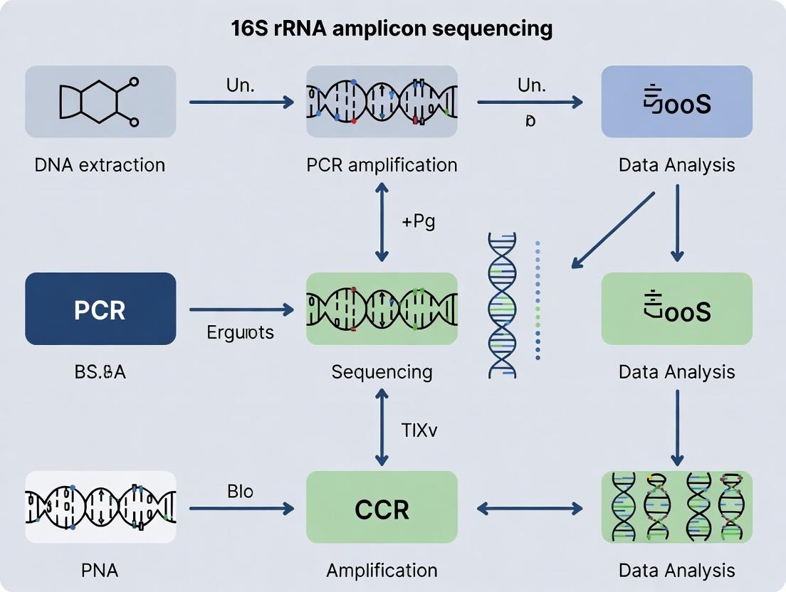
Within a 16S rRNA amplicon sequencing workflow for microbial ecology research, library preparation and indexing are critical steps that transform PCR-amplified target regions into sequencer-ready libraries. The choice of sequencing platform (e.g., Illumina or Ion Torrent) subsequently dictates the scale, read architecture, and analytical approach. This Application Note details protocols and considerations for this phase, enabling robust community profiling.
Library Preparation and Indexing: Core Principles
Following amplification of hypervariable regions (e.g., V3-V4), PCR products must be prepared into a sequencing library. This involves:
- Adapter Ligation/Attachment: Adding platform-specific oligonucleotide adapters that contain sequencing primer binding sites.
- Indexing (Barcoding): Incorporating unique molecular identifiers (indices/barcodes) via a second, shorter PCR to allow multiplexing of multiple samples in a single sequencing run.
- Clean-up and Normalization: Purifying the final library and quantifying/pooling samples at equimolar ratios.
Detailed Protocol: Dual-Index Library Preparation for Illumina MiSeq
Objective: To prepare indexed amplicon libraries from purified 16S rRNA gene PCR products for sequencing on an Illumina MiSeq system.
Materials:
- Purified 16S rRNA amplicon (e.g., ~550 bp V3-V4 product).
- Indexing Primers: Nextera XT Index Kit v2 (Illumina) primers (i5 and i7).
- High-Fidelity DNA Polymerase (e.g., KAPA HiFi HotStart ReadyMix).
- AMPure XP beads (Beckman Coulter).
- Tris-HCl (10 mM, pH 8.5).
- Quantification kit (e.g., Qubit dsDNA HS Assay).
- Fragment Analyzer or Bioanalyzer (Agilent).
Methodology:
- Index PCR Setup:
- In a 50 µL reaction, combine:
- 25 µL 2X High-Fidelity PCR Master Mix.
- 5 µL Forward (i5) Unique Index Primer.
- 5 µL Reverse (i7) Unique Index Primer.
- 5 µL (~10-50 ng) Purified Amplicon DNA.
- 10 µL PCR-grade water.
- Cycling Conditions: 95°C for 3 min; 8 cycles of: 95°C for 30s, 55°C for 30s, 72°C for 30s; final extension 72°C for 5 min; hold at 4°C.
- In a 50 µL reaction, combine:
PCR Clean-up:
- Vortex AMPure XP beads thoroughly. Add 50 µL (1.0x ratio) of beads to the 50 µL PCR reaction. Mix thoroughly.
- Incubate for 5 min at room temperature.
- Place on a magnetic stand for 2 min until clear. Discard supernatant.
- With tube on magnet, wash beads twice with 200 µL fresh 80% ethanol. Air dry for 5 min.
- Remove from magnet. Elute DNA in 52.5 µL Tris-HCl buffer. Mix, incubate 2 min, place on magnet, and transfer 50 µL of clean library to a new tube.
Library Quantification & Normalization:
- Quantify each library using the Qubit dsDNA HS Assay.
- Assess library size distribution using a Fragment Analyzer (expected peak ~630 bp including adapters).
- Dilute each library to 4 nM based on concentration and average size.
- Pool 5 µL of each 4 nM library to create the final multiplexed pool.
Denaturation & Dilution:
- Denature the pooled library with 0.2 N NaOH. Dilute to a final loading concentration of 8 pM (with 10% PhiX control) in HT1 buffer.
Sequencing Platform Comparison: Illumina vs. Ion Torrent
Table 1: Key Quantitative and Operational Parameters for Modern Sequencing Platforms in 16S rRNA Sequencing.
| Parameter | Illumina MiSeq System | Ion Torrent Ion GeneStudio S5 System |
|---|---|---|
| Core Technology | Reversible dye-terminator sequencing-by-synthesis (SBS) | Semiconductor-based detection of hydrogen ions released during DNA synthesis |
| Read Length (Max) | 2 x 300 bp (paired-end) | Up to 600 bp (single-end) |
| Output per Run | Up to 15 Gb | Up to 15 Gb (varies with chip) |
| Typical Run Time | 24-56 hours (for 2x300) | 2.5-5 hours |
| Multiplexing Capacity | Very High (≥384 samples via dual indexing) | High (≤96 samples with barcoding) |
| Key Strength for 16S | High accuracy (<0.1% error rate), high multiplexing, standardized protocols | Fast turnaround, lower upfront instrument cost |
| Key Limitation for 16S | Longer run time, higher cost per run | Higher error rates in homopolymer regions, shorter read lengths limiting some hypervariable region coverage |
Experimental Protocol: Library Preparation for Ion Torrent Sequencing
Objective: To prepare amplicon libraries from purified 16S rRNA gene PCR products for sequencing on an Ion Torrent S5 system.
Materials:
- Purified 16S rRNA amplicon.
- Ion Code Barcodes: Ion Xpress Barcode Adapters.
- Ion Plus Fragment Library Kit.
- NEBNext Ultra II FS DNA Module (for shearing, if required).
- Agencourt AMPure XP beads.
- Ion Library TaqMan Quantitation Kit.
Methodology:
- Blunt Ending & Adapter Ligation (if using full adapter ligation workflow):
- If the amplicon is >600 bp, shear DNA to ~450 bp using a focused ultrasonicator.
- Perform end-repair to create blunt ends using the provided enzymes.
- Ligate Ion-specific adapters, which include the barcode sequences, to the blunt-ended fragments.
- Barcoded Amplification (Common Method):
- Perform a limited-cycle (6-10 cycles) PCR using primers that have the Ion Torrent adapter sequences (A and P1) and the sample-specific barcode sequences.
- Use Platinum PCR SuperMix High Fidelity.
- Size Selection & Clean-up:
- Purify the PCR product twice using AMPure XP beads (0.8x ratio followed by 1.4x ratio) to remove primer dimers and select the correct library size.
- Quantification & Template Preparation:
- Quantify the library using the Ion Library TaqMan Quantitation Kit.
- Dilute the library to 50 pM for subsequent emulsion PCR (Ion Chef system automates template preparation).
Visualizing the Workflow
Title: Library Prep and Sequencing Platform Workflow
Title: Sequencing Chemistry Comparison
The Scientist's Toolkit: Research Reagent Solutions
Table 2: Essential Materials for Library Preparation and Sequencing.
| Item | Function & Relevance to 16S Workflow |
|---|---|
| Nextera XT Index Kit v2 (Illumina) | Contains unique dual index (i5 & i7) primer sets for high-level multiplexing with minimal index hopping. Essential for Illumina 16S studies. |
| Ion Code Barcodes (Thermo Fisher) | Pre-designed, balanced barcode sets optimized for Ion Torrent sequencing, enabling sample pooling. |
| KAPA HiFi HotStart ReadyMix | High-fidelity polymerase for index PCR, minimizing errors in barcode and adapter sequences. |
| AMPure XP Beads (Beckman Coulter) | Solid-phase reversible immobilization (SPRI) magnetic beads for size-selective clean-up and purification of libraries. |
| Qubit dsDNA HS Assay Kit | Fluorometric quantification specific to double-stranded DNA, critical for accurate library normalization before pooling. |
| PhiX Control v3 (Illumina) | Sequencer control library; adding 10-20% improves low-diversity amplicon run performance by providing sequence heterogeneity during cluster calling. |
| Ion Chef System & Reagents | Automated instrument and companion kits for templating (emulsion PCR) and chip loading for Ion Torrent systems, ensuring reproducibility. |
| Agilent High Sensitivity DNA Kit | For use with a Bioanalyzer to assess library fragment size distribution and detect adapter dimer contamination. |
Following meticulous sample collection, DNA extraction, PCR amplification, and library preparation, the raw data from high-throughput sequencing must be computationally processed to generate accurate, high-quality microbial community profiles. This phase is critical for transitioning from raw sequencing reads to meaningful biological sequences, directly impacting all downstream ecological analyses, including alpha/beta diversity, differential abundance, and biomarker discovery in drug development research.
Application Notes
Demultiplexing assigns each raw sequencing read to its sample of origin using unique barcode sequences added during library preparation. Modern tools like bcl2fastq (Illumina) or q2-demux (QIIME 2) perform this step with high accuracy, but barcode errors can lead to sample misassignment.
Adapter & Primer Trimming is essential as residual sequencing adapters and the conserved primer sequences used in PCR can interfere with downstream analysis, causing misalignment or chimeric artifacts.
Quality Filtering removes low-quality sequences and reads of inappropriate length, which are often the source of spurious OTUs/ASVs. The stringency of this step must be balanced to retain sufficient sequencing depth for statistical power while removing technical noise. Current consensus favors retaining reads with an expected error rate below 1% (e.g., Q-score ≥ 20 over most of the read).
Table 1: Comparison of Key Bioinformatics Tools for 16S rRNA Data Processing
| Tool / Platform | Primary Function | Key Algorithm/Feature | Typical Input | Typical Output |
|---|---|---|---|---|
| QIIME 2 (q2-demux) | Demultiplexing, visualization | Empirical quality plots, summarization | Raw FASTQ + barcodes | Demultiplexed FASTQ, quality reports |
| Cutadapt | Adapter/ primer trimming | Overlap alignment; error tolerance | FASTQ files | Trimmed FASTQ files |
| DADA2 (within QIIME2/R) | Quality filtering, denoising, chimera removal | Error model learning, ASV inference | Trimmed FASTQ | Amplicon Sequence Variants (ASVs) table |
| UNOISE3 (USEARCH) | Denoising, chimera removal | Clustering by abundance, error correction | Quality-filtered FASTQ | Zero-radius OTUs (ZOTUs) |
| fastp | All-in-one trimming & filtering | Adaptive quality trimming, duplication analysis | Raw FASTQ | Cleaned FASTQ, HTML report |
Table 2: Impact of Quality Filtering Parameters on Read Retention
| Filtering Parameter | Common Setting | Typical Read Loss | Purpose & Rationale |
|---|---|---|---|
| Max Expected Errors (--max-ee) | 1.0 for forward, 2.0 for reverse reads | 10-25% | Removes reads with an unacceptably high probability of containing errors. |
| Minimum Length (--trunc-len) | e.g., 220 bp (F), 200 bp (R) | 5-20% | Ensures reads cover a consistent, overlapping region for merging. |
| Quality Score Threshold (--qtrim) | Q ≥ 20 (Phred scale) | 15-30% | Trims low-quality bases from ends to improve overall read quality. |
| Chimera Removal | e.g., DADA2's removeBimeraDenovo |
5-15% | Eliminates artificial sequences formed from two+ parent sequences during PCR. |
Experimental Protocols
Protocol 1: Demultiplexing with QIIME 2 (2024.2)
- Prepare Manifest File: Create a comma-separated file with columns: sample-id, absolute-filepath, direction. Specify forward and reverse reads for paired-end data.
- Import Data: Use the
q2 tools importcommand with theSampleData[PairedEndSequencesWithQuality]type. - Summarize: Generate an interactive quality plot:
qiime demux summarize --i-data your-data.qza --o-visualization demux.qzv. - View Report: Open
demux.qzvin QIIME 2 View to inspect read counts per sample and quality scores across base positions, guiding trimming parameters.
Protocol 2: Trimming and Quality Filtering with DADA2 in R This protocol performs integrated trimming, filtering, denoising, and chimera removal.
- Install & Load: Install
dada2from Bioconductor. Load library:library(dada2). - Set Paths & Inspect Quality: Point to demultiplexed FASTQ files. Use
plotQualityProfile(fnFs[1:2])to visualize quality trends and decide trim positions. - Filter and Trim:
- Learn Error Rates & Dereplicate: Model the error rates (
learnErrors) and dereplicate identical reads (derepFastq). - Infer ASVs & Merge Pairs: Run the core sample inference algorithm (
dada) on each sample, then merge paired reads (mergePairs). - Remove Chimeras: Construct a sequence table and remove chimeras:
seqtab.nochim <- removeBimeraDenovo(seqtab, method="consensus", multithread=TRUE). - Track Reads: Monitor read retention through the pipeline using the
outmatrix and chimera removal stats.
Visualizations
Title: 16S rRNA Bioinformatics Pre-processing Workflow
Title: Logical Decision Tree for Read Filtering
The Scientist's Toolkit
Table 3: Essential Research Reagent Solutions & Computational Resources
| Item / Resource | Function in Pipeline | Example / Specification |
|---|---|---|
| High-Performance Computing (HPC) Cluster or Cloud Instance | Provides the necessary CPU, RAM, and storage for processing large sequencing datasets. | AWS EC2 (e.g., m5.4xlarge), Google Cloud, or local HPC with ≥ 16 cores & 64 GB RAM. |
| Containerized Software (Docker/Singularity Images) | Ensures reproducibility by packaging the exact software environment (versions, dependencies). | QIIME 2 Core distribution image, DADA2 RStudio container. |
| Sample Sheet (CSV File) | Maps sample identifiers to barcode sequences for demultiplexing; critical metadata. | Must match the format required by the demultiplexing tool (e.g., for bcl2fastq or QIIME 2). |
| Reference Databases for Contaminant Filtering | Identifies and removes non-target sequences (e.g., host DNA, phiX control). | Genome of host organism (e.g., human GRCh38), phiX174 genome. |
| Bioinformatics Pipeline Manager | Automates and documents the workflow, ensuring consistency and traceability. | Nextflow, Snakemake, or QIIME 2 pipelines. |
| Quality Report Visualizer | Allows interactive inspection of quality metrics to inform parameter decisions. | QIIME 2 View, MultiQC, fastp HTML reports. |
In 16S rRNA amplicon sequencing workflows for microbial ecology research, the bioinformatic step of grouping sequences into biologically relevant units is foundational. This phase determines the resolution at which microbial diversity is assessed, directly impacting downstream ecological inferences. The choice is fundamentally between two paradigms: Operational Taxonomic Units (OTUs), clustered based on a fixed sequence similarity threshold (typically 97%), and Amplicon Sequence Variants (ASVs), which are resolved to a single-nucleotide difference without imposing an arbitrary threshold. This protocol details the application and selection of traditional OTU clustering methods versus modern ASV inference algorithms like DADA2 and Deblur within a thesis focused on robust, reproducible microbial ecology research.
Comparative Analysis of Clustering Methods
Table 1: Core Algorithmic Comparison of Clustering Methods
| Feature | Traditional OTU Clustering (e.g., VSEARCH, UPARSE) | DADA2 (Divisive Amplicon Denoising Algorithm) | Deblur |
|---|---|---|---|
| Primary Output | OTUs (clusters at % identity) | Amplicon Sequence Variants (ASVs) | Amplicon Sequence Variants (ASVs) |
| Resolution | Typically 97% similarity; groups sequences. | Single-nucleotide; distinguishes sequences. | Single-nucleotide; distinguishes sequences. |
| Error Model | Relies on clustering to dampen errors. | Parametric error model learned from data. | A static, per-position expected error profile. |
| Chimera Removal | Separate step post-clustering (e.g., UCHIME). | Integrated into the denoising algorithm. | Separate step using empirical rules post-denoisin |
| Denoising Approach | Heuristic clustering & centroid selection. | Divisive partitioning; reads partitioned into sequence bins. | Iterative read subtraction based on error profiles. |
| Input Preference | Dereplicated sequences, often quality-filtered. | Quality-filtered reads (fastq). | Quality-filtered reads (fastq). |
| Computational Demand | Moderate. | High (especially for large datasets). | Moderate to High. |
| Key Advantage | Long history, well-understood, less computationally intensive for very large datasets. | High resolution, reduced false positives, excellent for strain-level tracking. | Fast, produces similar results to DADA2, streamlin workflow. |
| Key Limitation | Merges real biological variation, resolution loss. | Can be sensitive to parameter tuning, slower. | May be overly aggressive in some environments. |
Table 2: Practical Performance Metrics (Generalized from Recent Benchmarks)
| Metric | Traditional OTU (97%) | DADA2 | Deblur | Notes |
|---|---|---|---|---|
| Perceived Richness | Lowest | Highest | High | ASV methods recover more unique sequences. |
| Spurious OTU/ASV Control | Moderate (errors clustered) | High (denoising) | High (denoising) | ASV methods better distinguish errors from rare biospher |
| Reproducibility | Moderate | High | High | ASV results are more consistent across runs and analyses. |
| Runtime (on 10M reads) | ~1-2 hours | ~3-6 hours | ~2-4 hours | Varies significantly with hardware and dataset complexity. |
| Downstream Beta-Diversity Fidelity | Good | Excellent | Excellent | ASVs often yield more robust ecological distinctions. |
Detailed Experimental Protocols
Protocol 1: Traditional OTU Clustering with VSEARCH
Objective: To cluster quality-filtered sequences into 97% OTUs and generate an OTU table. Input: Merged, quality-filtered, and dereplicated FASTA files (from Phase 5: Chimera Removal). Software: VSEARCH (v2.26.0+).
Dereplication (if not done previously):
OTU Clustering (at 97% identity):
Chimera Filtering (de novo):
Map Reads to OTUs:
Protocol 2: ASV Inference using DADA2 (in R)
Objective: To infer exact Amplicon Sequence Variants from trimmed, filtered FASTQ files. Input: Paired-end, quality-trimmed FASTQ files (from Phase 3: Quality Control & Trimming). Software/R Package: DADA2 (v1.30.0+).
Load library and set path:
Learn error rates: Model the sequencing error profile from a subset of data.
Dereplication and Sample Inference: Core denoising step.
Merge paired reads: Combine forward and reverse reads.
Construct sequence table and remove chimeras:
Protocol 3: ASV Inference using Deblur (in QIIME 2)
Objective: To generate an ASV table via a rapid, read-subtraction-based denoising approach.
Input: Imported and demultiplexed paired-end sequences in QIIME 2 artifact format (.qza).
Software: QIIME 2 (v2024.5+) with deblur plugin.
Join paired-end reads:
Quality filter (strictly):
Run Deblur (key step): Uses a positive (retain) trim length.
Export for analysis:
Visualizations
Diagram 1: ASV/OTU Clustering Workflow Decision Tree
Diagram 2: Conceptual Resolution of OTUs vs ASVs
The Scientist's Toolkit: Research Reagent Solutions
Table 3: Essential Bioinformatics Tools & Resources for Clustering
| Item | Function/Benefit | Example/Version |
|---|---|---|
| QIIME 2 | Comprehensive, reproducible microbiome analysis platform. Integrates DADA2, Deblur, VSEARCH. | qiime2-2024.5 |
| DADA2 R Package | Specialized R package for accurate ASV inference using a parametric error model. | v1.30.0 |
| VSEARCH | Open-source, 64-bit alternative to USEARCH for OTU clustering, chimera detection, and read merging. | v2.26.0 |
| Cutadapt | Critical for prior trimming of primers/adapter sequences, ensuring clean input for clustering. | v4.6 |
| Silva / GTDB Database | Curated 16S rRNA databases for taxonomic assignment of OTU/ASV sequences post-clustering. | Silva v138.1, GTDB r220 |
| High-Performance Computing (HPC) Cluster | Necessary for processing large datasets with memory-intensive algorithms like DADA2. | SLURM/SGE |
| Conda/Bioconda | Package manager for creating isolated, reproducible software environments for analysis. | Miniconda3 |
| Snakemake/Nextflow | Workflow management systems to automate, scale, and reproduce the entire analysis pipeline. | Snakemake v7.32 |
| Positive Control Mock Community | Defined genomic mixture (e.g., ZymoBIOMICS) to benchmark pipeline accuracy and sensitivity. | Zymo D6300 |
Within the comprehensive 16S rRNA amplicon sequencing workflow for microbial ecology research, taxonomy assignment represents the critical juncture where processed sequence data is translated into biological meaning. This phase involves comparing representative amplicon sequence variants (ASVs) or operational taxonomic units (OTUs) against curated reference databases—primarily SILVA, Greengenes, and the Ribosomal Database Project (RDP)—to assign microbial identities at various taxonomic ranks. The choice of database and algorithm directly influences downstream ecological interpretations, making this a pivotal step in thesis research linking microbial community structure to function.
Database Comparison and Selection
The selection of a reference database is a fundamental decision that impacts taxonomic resolution, accuracy, and comparability with published studies. Key characteristics of the three major databases are summarized below.
Table 1: Comparison of Major 16S rRNA Reference Databases (Current as of 2024)
| Feature | SILVA | Greengenes | RDP |
|---|---|---|---|
| Current Version | SILVA 138.1 (SSU Ref NR) | gg138 (May 2013) | RDP Release 11, Update 11 (Sep 2023) |
| Last Major Update | 2020 | 2013 | 2023 |
| Primary Curation | Semi-automated, manually refined | Automated, then manually curated | Automated with manual review |
| Alignment & Taxonomy | Aligned via SINA; consistent taxonomy | Inferred alignment; taxonomy may vary | Aligned with Infernal; RDP taxonomy |
| Number of Quality-filtered Sequences | ~2.7 million (Ref NR) | ~1.3 million | ~4.2 million (16S seqs) |
| Taxonomy Hierarchy | Domain, Phylum, Class, Order, Family, Genus, Species | Domain, Phylum, Class, Order, Family, Genus | Domain, Phylum, Class, Order, Family, Genus |
| Primary File Formats | .fasta, .arb |
.fasta, .txt taxonomy |
.fasta, .align, .taxonomy |
| Strengths | Comprehensive, actively updated, includes eukaryotes; widely used in marine & European studies. | Historical standard; high comparability with older human microbiome studies. | Frequently updated; includes fungal LSU; well-integrated with Classifier tool. |
| Limitations | Large size can increase computational burden; occasional inconsistencies in novel taxa. | No longer actively updated; may miss newer taxa. | Primarily focused on cultivable strains; may have fewer environmental sequences. |
| Recommended Use Case | General-purpose, especially for environmental/non-human samples and recent studies. | For direct comparison with legacy human microbiome data (e.g., from QIIME 1). | When using the RDP Classifier tool; for studies including fungi. |
Detailed Protocols
Protocol 1: Taxonomy Assignment with QIIME 2 and SILVA
This protocol details assigning taxonomy to ASVs using QIIME 2’s q2-feature-classifier plugin and a pre-trained SILVA classifier.
Pre-requisites:
- QIIME 2 environment (version 2024.2 or later).
- Representative sequences file (
rep-seqs.qza) from DADA2 or deblur. - Download the SILVA 138.1 NR99 classifier trained on the V4 region (or your specific region) from the QIIME 2 Data Resources page.
Procedure:
- Import the classifier: Ensure the downloaded classifier (
.qza) is in your working directory. Execute taxonomy assignment:
Generate a visual summary:
View the
taxonomy.qzvin the QIIME 2 View to see the assignment per feature and its confidence.
- Import the classifier: Ensure the downloaded classifier (
Critical Parameters:
- Classifier Specificity: Use the "99%" or "97%" identity classifiers based on desired resolution. The "NR" (non-redundant) version is recommended.
- Read Orientation: Ensure your sequences are in the same orientation (typically forward) as the classifier training data.
- Confidence Threshold: The default confidence is 0.7. This can be adjusted later during filtering, not during the initial classification.
Protocol 2: Taxonomy Assignment with DADA2/RDP in R
This protocol performs taxonomy assignment directly within the DADA2 pipeline using the RDP reference database.
Pre-requisites:
- R environment with
dada2andphyloseqpackages installed. - ASV sequence table and representative sequence list from the
dada2::dada()andmergePairs()steps.
- R environment with
Procedure:
Critical Parameters:
tryRC=TRUE: Crucial as amplicon orientation is not always guaranteed.minBoot: The minimum bootstrap confidence for assigning a taxonomic rank (default=50). Increasing this value (e.g., to 80) increases stringency but yields more unassigned labels.- Species assignment is often performed with a separate, often SILVA-derived, database as RDP's species-level training is limited.
Protocol 3: Cross-Validation with Multiple Databases
For robust thesis findings, validating assignments across databases is recommended.
Procedure:
- Perform taxonomy assignment using Protocol 1 (SILVA) and Protocol 2 (RDP) on the same set of representative sequences.
- For Greengenes, use the corresponding QIIME 2 classifier or the
assignTaxonomy()function with the Greengenes reference file (gg_13_8_train_set_97.fa.gz). - Merge the results into a comparative table using a custom R or Python script, tracking assignments at the phylum and genus levels.
Analysis:
- Calculate the percentage agreement between databases for dominant taxa (>1% abundance).
- Flag taxa with discordant assignments (e.g., different phylum) for manual inspection via BLASTn against the NCBI nt database.
- Decide on a conservative assignment based on consensus and public sequence similarity.
Workflow Visualization
Taxonomy Assignment and Curation Workflow
The Scientist's Toolkit
Table 2: Essential Research Reagents & Resources for Taxonomy Assignment
| Item | Function & Description | Example/Format |
|---|---|---|
| Curated Reference Database | Provides the gold-standard set of classified 16S sequences for comparison. Choice dictates taxonomic nomenclature and coverage. | SILVA SSU Ref NR 138.1 .fasta; Greengenes 13_8 99%_otus.fasta; RDP RDP_16S_v18.fa |
| Pre-trained Classifier | A machine-learning model (often Naive Bayes) trained on a specific database and hypervariable region, enabling rapid classification. | QIIME2 compatible .qza files for V4/V3-V4 regions. |
| Species Assignment Database | A supplementary database focused on full-length 16S sequences for finer, species-level taxonomic calls. | silva_species_assignment_v138.1.fa.gz |
| Taxonomy Mapping File | A tab-separated file linking reference sequence identifiers to their full taxonomic path. | taxonomy.tsv or *.tax file. |
| Negative Control Database | A curated list of common contaminant sequences (e.g., from kits, human skin) for post-assignment filtering. | decontam package R list or contaminants.fasta |
| BLAST+ Suite | Command-line tools for manual validation of ambiguous ASVs against the NCBI non-redundant database. | blastn executable and locally formatted nt database. |
| Computational Environment | A reproducible environment with necessary bioinformatics tools and dependencies. | QIIME 2 Conda environment, RStudio with dada2, phyloseq, DECIPHER. |
| High-Performance Compute (HPC) Access | Essential for processing large datasets or training custom classifiers on full databases. | Slurm or PBS job scheduler access with sufficient RAM (≥64 GB). |
Application Notes
Following bioinformatic processing of 16S rRNA amplicon sequences (Phases 6 & 7), downstream analysis translates feature tables and phylogenetic trees into biological insights. This phase is critical for testing hypotheses about microbial community structure and function within a microbial ecology thesis.
Core Analytical Objectives:
- Alpha Diversity: Quantifies the richness, evenness, and diversity of species within a single sample. It is used to test hypotheses about local species diversity under different conditions (e.g., diseased vs. healthy states).
- Beta Diversity: Measures compositional differences between microbial communities. It tests hypotheses regarding whether sample groupings (e.g., by treatment) harbor distinct microbial ecosystems.
- Differential Abundance (DA): Identifies specific taxa (e.g., at the genus or species level) whose abundances differ significantly between predefined sample groups. This moves from community-level to taxon-specific hypotheses.
- Visualization: Communicates complex multivariate data and statistical findings in an accessible format, enabling intuitive interpretation and hypothesis generation.
Current Challenges & Considerations: Recent best practices emphasize the compositional nature of amplicon data, advising the use of appropriate log-ratio transformations for multivariate and differential abundance analyses to avoid spurious correlations. The field is moving towards robust, standardized workflows that account for data sparsity and high variability.
Protocols
Protocol: Alpha Diversity Analysis with QIIME 2
Objective: To calculate and statistically compare within-sample microbial diversity indices.
Materials:
- QIIME 2 core distribution (2024.5 or later)
- Input: QIIME 2 artifact of type
FeatureTable[Frequency](rarefied) andFeatureData[Sequence] - R software with
ggplot2andveganpackages (for external plotting/stats)
Procedure:
- Rarefaction: Rarefy the feature table to an even sampling depth to eliminate sequencing effort as a confounding variable.
Calculate Alpha Diversity: Compute observed features (richness) and the Shannon diversity index (evenness).
Statistical Comparison: Use the Kruskal-Wallis test to compare diversity across groups.
Protocol: Beta Diversity Analysis & PERMANOVA
Objective: To visualize and test for significant differences in community composition between sample groups.
Materials:
- QIIME 2 core distribution
- R software with
phyloseq,vegan,ggplot2packages
Procedure:
- Generate Distance Matrices: Calculate pairwise community dissimilarities using phylogeny-aware (UniFrac) and abundance-based (Bray-Curtis) metrics.
Dimensionality Reduction: Perform Principal Coordinates Analysis (PCoA) for visualization.
Statistical Testing: Perform Permutational Multivariate Analysis of Variance (PERMANOVA) using
adonis2in R to test if group centroids are significantly different.
Protocol: Differential Abundance Analysis with ANCOM-BC
Objective: To identify taxa with significantly different abundances across groups, accounting for compositionality.
Materials:
- R software (v4.3.0+) with
ANCOMBCandphyloseqpackages.
Procedure:
- Data Preparation: Create a
phyloseqobject from the feature table, taxonomy, and metadata.
Run ANCOM-BC: This method estimates unknown sampling fractions and corrects bias for false discovery rate control.
Interpret Results: Extract the
resobject containing log-fold changes, standard errors, p-values, and q-values for each taxon and contrast.
Data Presentation
Table 1: Common Alpha Diversity Indices in Microbial Ecology
| Index | Formula | Sensitivity | Interpretation |
|---|---|---|---|
| Observed Features | S | Richness Only | Simple count of unique ASVs/OTUs. |
| Shannon Index | H' = -Σ(pi * ln pi) | Richness & Evenness | Increases with more taxa and more even distribution. |
| Faith's PD | Σ(branch lengths) | Phylogenetic Richness | Sum of phylogenetic branch lengths present in a sample. |
| Pielou's Evenness | J' = H' / ln(S) | Evenness Only | How evenly abundances are distributed (0 to 1). |
Table 2: Comparison of Differential Abundance Methods for 16S Data
| Method | Principle | Compositionally Aware? | Handles Zeros? | Key Software |
|---|---|---|---|---|
| ANCOM-BC | Linear model with bias correction & FDR control. | Yes (log-ratio) | Yes (prev. filter) | ANCOMBC (R) |
| DESeq2 | Negative binomial GLM with shrinkage. | No (uses raw counts) | Robust with low counts | DESeq2 (R) |
| LEfSe | K-W/R test followed by LDA effect size. | No (rel. abundance) | Moderate | Galaxy, Huttenhower Lab |
| ALDEx2 | Monte Carlo sampling from a Dirichlet prior. | Yes (CLR transform) | Excellent | ALDEx2 (R) |
Visualization Diagrams
Diagram Title: Downstream Analysis Core Workflow
Diagram Title: Diversity Metric Selection Guide
The Scientist's Toolkit
Table 3: Essential Research Reagent Solutions & Tools for Downstream Analysis
| Item | Function in Analysis | Example Product/Software |
|---|---|---|
| Statistical Software (R/Python) | Provides environment for data manipulation, statistical testing, and custom visualization. | R (v4.3.0+), Python (v3.9+) |
| Microbiome Analysis Packages | Specialized libraries implementing diversity calculations, compositional transforms, and DA methods. | R: phyloseq, vegan, ANCOMBC, microbiome. Python: scikit-bio, gneiss. |
| Visualization Libraries | Generate publication-quality plots (boxplots, PCoA, heatmaps, cladograms). | R: ggplot2, ComplexHeatmap. Python: matplotlib, seaborn. |
| High-Performance Computing (HPC) Access | Enables processing of large distance matrices and permutation tests (e.g., 10,000+ PERMANOVA iterations). | University HPC clusters, cloud computing (AWS, GCP). |
| Interactive Visualization Tools | Allows exploratory data sharing and interrogation by collaborators without coding. | Qiita, Pavian, Krona, Emperor. |
Solving Common 16S Challenges: A Troubleshooting Guide for Reliable Data
Within the context of 16S rRNA amplicon sequencing workflows for microbial ecology research, contamination from laboratory reagents, kits, and the environment presents a critical challenge. These contaminants can obscure true biological signals, particularly in low-biomass samples, leading to erroneous ecological conclusions and compromised data integrity in both academic research and drug development pipelines. This document outlines the sources, identification, and mitigation strategies for these contaminants through detailed application notes and protocols.
The following tables summarize commonly reported contaminant taxa and their frequencies, derived from recent literature and controlled studies.
Table 1: Common Bacterial Genera Identified as Reagent & Kit Contaminants in 16S rRNA Studies
| Genus | Typical Source | Reported Frequency in Negative Controls (%) | Notes |
|---|---|---|---|
| Pseudomonas | Molecular grade water, PCR reagents | 65-80 | Often dominates water and buffer-associated contaminant profiles. |
| Acinetobacter | DNA extraction kits, plasticware | 45-60 | Common in silica membrane-based kits. |
| Burkholderia | PCR master mixes, polymerases | 20-35 | Persistent in some enzyme preparations. |
| Propionibacterium/Cutibacterium | Human skin, handling | 30-50 | More frequent in manually processed kits. |
| Ralstonia | Laboratory water systems, buffers | 50-70 | Prevalent in ultrapure water systems. |
| Staphylococcus | Human skin, aerosol | 15-30 | Correlates with level of human activity. |
Table 2: Impact of Environmental Controls on Observed OTUs
| Control Type | Mean OTUs Detected (SD) | Median Read Count | Primary Mitigation Strategy |
|---|---|---|---|
| Extraction Blank (no sample) | 18.5 (6.2) | 1,245 | Dedicated UV hood, dedicated reagents |
| PCR Negative Control (water) | 5.7 (2.1) | 302 | Aliquot enzymes, use UV-treated plasticware |
| Sequencer Carry-over Control | 12.3 (4.8) | 850 | Balanced library pooling, PhiX spike-in (>5%) |
| Laboratory Surface Swab | 45.2 (15.6) | 3,450 | Regular decontamination, HEPA filtration |
Experimental Protocols
Protocol 3.1: Systematic Contaminant Profiling for Laboratory Workflow
Objective: To create a laboratory-specific contaminant database by processing a complete set of negative controls alongside sample batches. Materials: See "The Scientist's Toolkit" below. Procedure:
- Batch Design: For each extraction batch of up to 22 samples, include:
- 2 extraction blanks (lysis buffer only).
- 1 mock community (positive control).
- 1 previously extracted sample (positive extraction control).
- Nucleic Acid Extraction:
- Perform extraction in a PCR workstation or laminar flow hood irradiated with UV light for 30 minutes prior to use.
- Use dedicated, aliquoted reagents for negative controls. Process controls first.
- Include a mechanical lysis step (bead beating) for blanks to account for kit-borne contaminants released under standard conditions.
- PCR Amplification:
- Amplify the V3-V4 hypervariable region of the 16S rRNA gene using primers 341F/806R with attached Illumina adapters.
- For each PCR plate, include a minimum of 3 no-template controls (NTCs) using UV-treated molecular grade water.
- Aliquot all PCR master mix components. Use a separate set of pipettes for control setup.
- Sequencing & Bioinformatics:
- Sequence on an Illumina MiSeq with a minimum of 20% PhiX spike-in to increase diversity.
- Process raw reads through DADA2 or QIIME 2 pipeline to generate amplicon sequence variants (ASVs).
- Contaminant Identification: Use the
decontampackage (R) in "frequency" mode, comparing the prevalence of ASVs in true samples versus the combined negative controls (extraction blanks + NTCs). ASVs with a statistically higher prevalence in negatives are designated contaminants. - Generate a lab-specific "contaminant blacklist" of ASVs for subsequent studies.
Protocol 3.2: Environmental Monitoring via Surface and Air Sampling
Objective: To quantify and identify environmental contaminants in the laboratory workspace. Procedure:
- Surface Sampling (Weekly):
- Moisten a sterile swab with sterile PBS.
- Swab a standardized area (e.g., 10x10 cm) of key surfaces: inside the PCR hood, extraction bench, pipette handles, and sequencing instrument loading bay.
- Place the swab tip in a tube with lysis buffer and process identically to a sample starting from Protocol 3.1, Step 2.
- Air Sampling (Monthly):
- Use a portable microbial air sampler.
- Collect 1000L of air onto a sterile membrane filter.
- Aseptically transfer the filter to lysis buffer and process.
- Data Integration: Compare ASVs from environmental samples to the contaminant blacklist and sample sets to identify potential infiltration points.
Visualization of Workflows and Relationships
Title: 16S Workflow Contaminant Control Pathway
Title: Contaminant Introduction and Impact Logic
The Scientist's Toolkit: Essential Research Reagent Solutions
Table 3: Key Materials for Contamination-Aware 16S rRNA Research
| Item | Function & Rationale | Contamination Control Feature |
|---|---|---|
| UV-treated Pipette Tips & Tubes | Sample and reagent handling. | Pre-sterilized via UV irradiation to degrade contaminating DNA. |
| Molecular Grade Water (Certified Nuclease-Free, DNA-Free) | Hydration of buffers, PCR setup, dilutions. | Tested via ultrasensitive PCR to ensure absence of bacterial DNA. |
| Aliquoted PCR Master Mix Components | DNA amplification. | Small, single-use aliquots prevent cross-contamination from repeated use of stock tubes. |
| Mock Microbial Community (e.g., ZymoBIOMICS) | Positive process control. | Defined composition validates sensitivity and detects bias; deviations indicate contamination or inhibition. |
| DNA/RNA Shield or Similar Preservation Buffer | Immediate sample preservation upon collection. | Inactivates nucleases and microbes, halting biomass changes and overgrowth of contaminants. |
| PCR Workstation with UV Decontamination | Primary workspace for reagent handling. | HEPA filtration removes airborne particles; UV light degrades contaminating nucleic acids on surfaces. |
| Barrier (Filter) Pipette Tips | All liquid handling. | Prevent aerosol carryover into pipette shaft, a major contamination vector. |
| Decontamination Solution (e.g., 10% Bleach, DNA Away) | Surface and equipment cleaning. | Degrades DNA/RNA between experimental procedures. More effective than ethanol alone. |
| High-Purity PCR Enzymes (e.g., recombinant, host-strain depleted) | DNA polymerase for amplification. | Sourced from strains lacking common contaminant genomes (e.g., Pseudomonas). |
In 16S rRNA gene amplicon sequencing, PCR artifacts are a primary source of bias, distorting the representation of true microbial community structure. Within the context of a comprehensive thesis on the 16S rRNA amplicon workflow in microbial ecology, this document details the origins, impacts, and mitigation strategies for three critical artifacts: chimeric sequences, primer binding bias, and differential amplification efficiency. These artifacts can confound ecological interpretations and compromise reproducibility, making their management essential for robust research and drug development targeting microbiomes.
Quantitative Impact of PCR Artifacts
The following table summarizes the typical prevalence and impact of key PCR artifacts in 16S rRNA sequencing studies, based on current literature.
Table 1: Prevalence and Impact of Major PCR Artifacts
| Artifact Type | Typical Frequency/Impact Range | Primary Consequence | Key Influencing Factors |
|---|---|---|---|
| Chimeric Sequences | 5% - 30% of reads (higher in complex communities) | Inflation of spurious OTUs/ASVs, false diversity | Cycle number, template concentration, polymerase, community complexity |
| Primer Binding Bias | >1000-fold variation in amplification efficiency between taxa | Skewed relative abundance, under-detection of taxa | Primer-template mismatches, GC content, secondary structure |
| Differential Amplification Efficiency | Efficiency (E) variance from 70% to 110% per taxon | Non-linear amplification, distortion of abundance ratios | Amplicon length, sequence context, polymerase fidelity |
Detailed Protocols and Application Notes
Protocol forIn SilicoPrimer Evaluation and Selection
Objective: To minimize primer binding bias through computational screening of primer pairs against a curated 16S rRNA database. Materials:
- Primer candidate sequences.
- SILVA or Greengenes reference database (latest version).
- Software: TestPrime (integrated in SILVA), ecoPCR, or PrimerProspector. Procedure:
- Database Preparation: Download the latest non-redundant SILVA SSU Ref NR dataset. Format for use with the chosen software (e.g.,
makeblastdbfor BLAST-based tools). - Mismatch Tolerance Definition: Set parameters for allowable mismatches (typical: 0-3 mismatches total, with no mismatches in the last 3-5 bases at the 3' end).
- In Silico PCR: Run the evaluation tool (e.g., TestPrime on the SILVA website) with your primer sequences and defined parameters against the target region (e.g., V4).
- Coverage Analysis: Calculate the percentage of target bacterial and archaeal sequences that are amplified in silico. Prioritize primer pairs with >90% coverage for common hypervariable regions.
- Bias Assessment: Analyze the taxonomic distribution of sequences that fail to amplify due to mismatches. Reject primer pairs that systematically exclude entire phyla of interest.
Protocol for Chimera Detection and Removal Using DADA2
Objective: To identify and remove chimeric sequences from FASTQ files post-sequencing. Materials:
- Demultiplexed paired-end FASTQ files.
- Computational environment with R and DADA2 installed. Procedure:
- Preprocessing: Follow standard DADA2 pipeline: quality filtering, error rate learning, dereplication, and sample inference.
- Chimera Identification: After merging paired reads and constructing the amplicon sequence variant (ASV) table, apply the
removeBimeraDenovofunction with themethod="consensus"parameter.
- Validation: Manually inspect removed sequences by aligning them to parent sequences using a tool like BLAST or visualizing in DECIPHER (
FindChimerasfunction). - Reporting: Document the percentage of reads identified as chimeric for each sample (typically 10-25%).
Protocol for Assessing Amplification Efficiency via qPCR Standard Curves
Objective: To quantify differential amplification efficiency across templates using a qPCR-based approach. Materials:
- Genomic DNA from 3-4 representative pure cultures spanning relevant phyla.
- Universal 16S rRNA gene primer pair.
- SYBR Green qPCR Master Mix.
- Real-time PCR instrument. Procedure:
- Template Serial Dilution: For each gDNA template, create a 5-log serial dilution series (e.g., from 10 ng/µL to 0.001 ng/µL).
- qPCR Run: Amplify each dilution in triplicate using the universal primer set and SYBR Green chemistry. Include no-template controls.
- Standard Curve Analysis: For each template, plot the mean Cq value against the log10 of the template concentration. The slope of the linear regression is used to calculate amplification efficiency (E): E = [10^(-1/slope)] - 1.
- Efficiency Comparison: Tabulate efficiencies. An ideal universal primer pair will yield E values within a narrow range (e.g., 95% ± 5%) across diverse templates. Larger variances indicate bias.
Diagrams
Title: PCR Artifact Generation and Mitigation Workflow
Title: Chimera Formation via Incomplete Extension
The Scientist's Toolkit: Research Reagent Solutions
Table 2: Essential Reagents and Kits for Artifact Mitigation
| Item | Function / Rationale | Example Product(s) |
|---|---|---|
| High-Fidelity DNA Polymerase | Reduces misincorporation errors and incomplete extensions that lead to chimeras. | Q5 Hot Start (NEB), Phusion Plus (Thermo), KAPA HiFi |
| Dual-Indexed Primers & Library Kits | Enables robust multiplexing with unique sample identifiers, reducing index hopping artifacts. | Illumina Nextera XT Index Kit, 16S Metagenomic Library Prep |
| Mock Microbial Community DNA | Validates entire workflow, providing known ratios to quantify primer bias and chimera rates. | ZymoBIOMICS Microbial Community Standard, ATCC MSA-1003 |
| PCR Inhibitor Removal Beads/Columns | Purifies environmental gDNA, ensuring consistent PCR efficiency across samples. | OneStep PCR Inhibitor Removal Kit (Zymo), SeraMag Beads |
| qPCR Master Mix with High Specificity | Allows accurate quantification of template and assessment of amplification efficiency bias. | SYBR Green Master Mix (Applied Biosystems), LightCycler 480 SYBR Green I |
| Uracil-DNA Glycosylase (UDG) | Controls carryover contamination from previous PCRs, reducing background artifacts. | Heat-labile UDG included in many one-step RT-PCR kits. |
Within 16S rRNA amplicon sequencing workflows for microbial ecology research, low-biomass samples present a significant challenge. These samples, characterized by a microbial load below typical detection thresholds (e.g., <10^4 microbial cells), are common in environments like sterile pharmaceuticals, cleanroom surfaces, indoor air, and certain human body sites (e.g., placenta, low-biomass tumors). The primary risks are false positives from exogenous contamination and false negatives due to insufficient template, which can severely compromise ecological inferences and drug product safety assessments. This application note details specialized considerations and validation protocols essential for reliable data generation.
Special Considerations and Challenges
- Contamination Dominance: Reagent-derived microbial DNA (from polymerases, kits, water) can constitute >90% of sequencing reads in ultra-low biomass samples.
- Inhibitor Sensitivity: Trace levels of inhibitors (e.g., cleaning agents, host biomolecules) have a disproportionate impact on amplification efficiency.
- Statistical Noise: Stochastic variation in early PCR cycles and library preparation can skew community profiles.
Table 1: Quantitative Risks in Low-Biomass 16S rRNA Sequencing
| Risk Factor | Typical Impact in Low-Biomass Context | Mitigation Strategy |
|---|---|---|
| Reagent Contamination | Can contribute 10^1 - 10^3 copies of 16S rRNA per µL of extraction kit eluent. | Use of sterilized, ultrapure reagents; inclusion of multiple negative controls. |
| Cross-Contamination | A single aerosolized cell can become the dominant signal. | Physical separation of pre- and post-PCR areas; use of dedicated equipment. |
| PCR Inhibition | 10x lower inhibitor concentration can cause 50% reduction in amplification yield. | Sample dilution, use of inhibitor-resistant polymerases, or additional purification. |
| Limit of Detection (LOD) | Often >10^2-10^3 copies of 16S gene per reaction, masking rarer taxa. | Increased template volume, technical replicates, optimized primer cocktails. |
Experimental Protocols
Protocol 1: Rigorous Negative Control Strategy
Purpose: To identify and computationally subtract contaminating operational taxonomic units (OTUs) derived from reagents and laboratory processes. Procedure:
- For every batch of samples processed, include at least three types of negative controls:
- Extraction Blank: Process a tube containing only the lysis buffer through the entire DNA extraction and library prep.
- Library Prep Blank: Use molecular-grade water as input during the library construction step.
- Sequencing Blank: Include a water-only well on the sequencing run.
- Process controls in the same physical location and using the same reagent lots as the true samples.
- Sequence all controls to the same depth as the samples (minimum 50,000 reads per control).
- Bioinformatic Subtraction: Any OTU present in the negative controls with a mean relative abundance greater than 1% of its mean abundance in the samples should be considered a potential contaminant and removed from the sample dataset.
Protocol 2: Inhibition Testing and Sample Processing
Purpose: To assess and overcome PCR inhibition in low-biomass extracts. Procedure:
- Spike-In Internal Control: During the lysis step, add a known, low quantity (e.g., 10^3 copies) of synthetic 16S rRNA gene from a non-native organism (e.g., Salmonella bongori) or a synthetic DNA standard.
- Perform qPCR on all sample extracts targeting both the spike-in and the total bacterial 16S rRNA gene.
- Calculate Inhibition: Compare the cycle threshold (Ct) value of the spike-in in the sample to its Ct in a clean water control. A delay of >2 Ct indicates significant inhibition.
- Remediation: For inhibited samples, either:
- Dilute the extract 1:10 and re-run qPCR, or
- Perform an additional clean-up step using a kit designed for inhibitor removal (e.g., OneStep PCR Inhibitor Removal Kit).
Protocol 3: Technical Replication for Validation
Purpose: To distinguish true signal from stochastic noise. Procedure:
- For each low-biomass sample, perform at least three independent library preparations from the same DNA extract.
- Sequence each replicate library on separate sequencing runs or lanes if possible.
- Validation Criteria: A taxon is considered confidently detected if it is present in ≥67% of the technical replicates with a non-zero read count. This filters out random PCR artifacts and index hopping events.
The Scientist's Toolkit
Table 2: Essential Research Reagent Solutions for Low-Biomass Work
| Item | Function in Low-Biomass Context |
|---|---|
| Ultrapure, DNA-Free Water (e.g., Invitrogen UltraPure) | Serves as the base for all reagents and dilutions, minimizing background DNA. |
| Sterile, Low-Binding Tips and Tubes | Reduces adhesion of microbial cells and DNA to plastic surfaces, maximizing recovery. |
| UV-Irradiated, PCR-Grade Reagents | Pre-sterilized enzymes and buffers decrease contaminant load from the assay itself. |
| Mock Community Standards (e.g., ZymoBIOMICS) | Validates entire workflow sensitivity and accuracy with known, low-input cell counts. |
| Inhibitor-Resistant Polymerase Mix (e.g., Phusion U Green) | Improves amplification robustness from challenging samples with trace inhibitors. |
| High-Sensitivity DNA Quantification Kit (e.g., Qubit HS dsDNA) | Accurately measures the often very low (<0.1 ng/µL) DNA concentrations. |
Workflow and Validation Diagrams
Low-Biomass 16S Workflow & Validation
Contaminant Subtraction Decision Tree
Within the 16S rRNA amplicon sequencing workflow for microbial ecology research, the steps of denoising and clustering are critical for transforming raw sequence reads into biologically meaningful Operational Taxonomic Units (OTUs) or Amplicon Sequence Variants (ASVs). The accuracy of downstream ecological inferences—diversity metrics, differential abundance, and biomarker discovery—is wholly dependent on the careful optimization of parameters during these bioinformatic steps. This protocol addresses common pitfalls and provides a standardized framework for parameter optimization, ensuring reproducible and robust results for researchers, scientists, and drug development professionals.
The following tables summarize core parameters for popular denoising and clustering tools, their typical default values, recommended optimization ranges, and their primary impact on output.
Table 1: Denoising Algorithm Parameters (DADA2, UNOISE3)
| Algorithm | Parameter | Default | Optimization Range | Impact on Output |
|---|---|---|---|---|
| DADA2 | maxEE (Expected Errors) |
2 (Fwd & Rev) | 1-5 | Higher values retain more reads but increase error rate. |
truncQ (Quality score truncation) |
2 | 2-20 | Lower values truncate more aggressively, potentially losing good sequence. | |
minLen (Minimum length) |
50 | 100-250 | Filters chimeras and primer-dimers; too high removes valid sequences. | |
pool (Pooling samples) |
FALSE | FALSE, pseudo, TRUE | TRUE increases sensitivity to rare variants but increases computational cost. |
|
| UNOISE3 | -minsize (Min cluster size) |
8 | 4-20 | Lower values detect rare ASVs but increase noise and chimeras. |
-unoise_alpha (Alpha parameter) |
2.0 | 1.0-4.0 | Controls rate of error correction; higher is more aggressive. |
Table 2: Clustering Algorithm Parameters (VSEARCH, CD-HIT)
| Algorithm | Parameter | Default | Optimization Range | Impact on Output |
|---|---|---|---|---|
| VSEARCH | --id (Identity threshold) |
0.97 | 0.95-0.99 | Defines OTU boundaries; lower increases alpha diversity, higher decreases it. |
--strand |
plus |
plus, both |
both increases matches but is computationally slower. |
|
--maxaccepts |
0 (unlimited) | 10-500 | Limits searches for speed; lower may miss some matches. | |
| CD-HIT | -c (Sequence identity) |
0.97 | 0.90-0.99 | Similar impact to VSEARCH --id. |
-n (Word length) |
5 | 4-6 | Lower increases sensitivity and time; higher reduces both. |
Application Notes & Detailed Protocols
Protocol 3.1: Systematic Parameter Optimization for DADA2
Objective: To empirically determine optimal maxEE and truncLen parameters for a given dataset.
Materials: Paired-end FASTQ files, R environment with DADA2 (≥1.28.0), high-performance computing access.
Procedure:
- Generate Parameter Matrix: Create a matrix testing
maxEE=c(1,2,3,4)andtruncLenpairs (e.g.,c(240,200),c(250,220),c(260,240)). - Run Iterative Denoising: For each parameter combination, run the standard DADA2 pipeline (
filterAndTrim(),learnErrors(),dada(),mergePairs(),makeSequenceTable()). - Metrics Collection: For each run, record: (a) Percentage of reads retained, (b) Number of inferred ASVs, (c) Estimated chimeras removed (%).
- Decision Point: Plot metrics against parameters. The optimal combination maximizes read retention while minimizing the rate of chimera formation (often identified by a knee-point in the curve). Avoid combinations where ASV count increases dramatically with small increases in
maxEE, indicating error inclusion.
Objective: To assess the sensitivity of downstream alpha and beta diversity results to OTU clustering identity threshold. Materials: Error-corrected sequence table (from DADA2 or UNOISE), VSEARCH (≥2.22.0), QIIME2 (2024.5) or R/phyloseq. Procedure:
- Multi-Threshold Clustering: Cluster the same sequence table at 97%, 98%, and 99% identity using VSEARCH (
--cluster_size). - Uniform Downstream Processing: Generate OTU tables, assign taxonomy using a consistent reference database (e.g., Silva 138.1), and construct phylogenetic trees.
- Diversity Analysis: Calculate core alpha diversity metrics (Observed, Shannon) and beta diversity metrics (Weighted/Unweighted UniFrac, Bray-Curtis) for each threshold.
- Statistical Comparison: For a defined sample grouping (e.g., Healthy vs. Diseased), perform PERMANOVA on each beta diversity matrix. Record the pseudo-F statistic and p-value.
- Interpretation: Optimal threshold is one where key ecological conclusions (e.g., significant separation between groups) are stable across small threshold variations. Instability indicates that results are artifact-prone.
Mandatory Visualizations
Title: 16S Workflow: Denoising and Clustering Steps with Pitfalls
Title: Parameter Optimization Feedback Loop
The Scientist's Toolkit: Research Reagent Solutions
Table 3: Essential Materials for Parameter Optimization Experiments
| Item | Function in Optimization | Example/Supplier |
|---|---|---|
| Mock Microbial Community DNA | Gold-standard control containing known abundances of bacterial strains. Used to calculate accuracy (recall, precision) of denoising/clustering parameters. | BEI Resources: HM-276D (ZymoBIOMICS Gut Microbiome Standard). |
| High-Performance Computing (HPC) Cluster Access | Enables parallel processing of multiple parameter combinations in a feasible timeframe. Essential for Protocol 3.1. | Local university cluster, AWS EC2, Google Cloud. |
| Bioinformatics Pipeline Managers | Tools to reliably orchestrate and reproduce multi-step parameter sweeps, capturing all software versions. | Nextflow, Snakemake. |
| Interactive Analysis Notebook | Environment for visualizing optimization metrics and making decisions. | RStudio with phyloseq, ggplot2; Jupyter with qiime2. |
| Curated Reference Database | Consistent taxonomic assignment is required to evaluate the biological realism of different parameter outputs. | SILVA, Greengenes, GTDB. Use a specific version (e.g., SILVA 138.1). |
| Data Visualization Library | Creates standard plots (knee-plots, stability curves) to compare parameter performance objectively. | R: ggplot2. Python: matplotlib, seaborn. |
Within the context of 16S rRNA amplicon sequencing workflows for microbial ecology and drug development research, a persistent challenge is the limited taxonomic resolution offered by short-read sequencing of this gene. While genus-level assignments are common, species- and strain-level discrimination is often necessary to understand functional potential, host-microbe interactions, and pathogenicity. This application note details current, advanced strategies to move beyond genus-level assignments, enhancing the biological insights derived from amplicon-based studies.
Core Strategies for Enhanced Resolution
Targeting Hypervariable Sub-Regions
Focusing sequencing effort on specific, more variable regions of the 16S gene (e.g., V4-V5, V3-V4, or V1-V2) can improve differentiation between closely related species.
Table 1: Resolution Power of Common 16S Primer Pairs
| Primer Pair (Region) | Average Amplicon Length (bp) | Typical Classification Depth | Key Advantage for Resolution |
|---|---|---|---|
| 27F-338R (V1-V2) | ~310 | Species-level for some taxa | High variability in V1-V2 |
| 338F-806R (V3-V4) | ~468 | Genus to Species | Good balance of length & info |
| 515F-926R (V4-V5) | ~411 | Genus | High accuracy, low error |
| 515F-806R (V4) | ~292 | Genus | Standardized, highly curated |
Utilizing Long-Read Sequencing Technologies
Platforms like PacBio SMRT and Oxford Nanopore enable full-length 16S rRNA gene sequencing (~1,500 bp), dramatically improving phylogenetic resolution.
Table 2: Comparison of Long-Read vs. Short-Read 16S Sequencing
| Metric | Illumina (Short-Read) | PacBio Hi-Fi (Long-Read) |
|---|---|---|
| Read Length | 250-300 bp | 1,300-1,600 bp |
| Estimated Error Rate | <0.1% | ~0.1% (after correction) |
| Cost per Sample | $20-$50 | $80-$150 |
| ASV/OTU Clustering | Required | Often unnecessary |
| Species-Level ID | Limited | Highly Improved |
Bioinformatics Pipelines & Custom Databases
Employing advanced algorithms and curated, specialized reference databases increases assignment accuracy.
Protocol 2.3.1: Custom Database Curation for Species-Level Assignment
- Source High-Quality Sequences: Download full-length 16S rRNA sequences from type strains in RefSeq or SILVA.
- Dereplicate and Cluster: Use
vsearch --derep_fulllengthand--cluster_sizeat 99% identity. - Taxonomy Annotation: Assign taxonomy using the GTDB (Genome Taxonomy Database) toolkit for consistent, genome-based nomenclature.
- Format for Classifier: Train a classifier (e.g., for QIIME 2, use
qiime feature-classifier fit-classifier-naive-bayes) on the curated reference sequences. - Validate: Test classifier performance on mock community data with known composition.
Analysis of Sub-Operational Taxonomic Units (sOTUs) / Amplicon Sequence Variants (ASVs)
Using denoising algorithms (DADA2, Deblur, UNOISE3) to infer exact biological sequences reduces errors and can reveal subtle genetic variations indicative of strain-level differences.
Protocol 2.4.1: DADA2 Pipeline for High-Resolution ASV Inference
- Filter and Trim: In R, use
dada2::filterAndTrim(trimLeft=10, truncLen=c(240,200), maxN=0, maxEE=c(2,2)). - Learn Error Rates:
learnErrors(..., nbases=1e8, multithread=TRUE). - Dereplication:
derepFastq(). - Sample Inference:
dada(derep, err=learned_error_rates, pool=TRUE)for sensitive detection of variants. - Merge Paired Reads:
mergePairs(... minOverlap=20). - Construct ASV Table:
makeSequenceTable()and remove chimeras withremoveBimeraDenovo(method="consensus"). - Taxonomy Assignment: Assign taxonomy using
assignTaxonomy(minBoot=80)with a species-level database (e.g., SILVA 138.1 with species delineation).
Complementary Functional Profiling
Predictive metagenomics (PICRUSt2, Tax4Fun2) and targeted functional gene amplicons can infer functional differences that taxonomic classification cannot.
Table 3: Tools for Functional Inference from 16S Data
| Tool | Input | Method | Output |
|---|---|---|---|
| PICRUSt2 | ASV Table | Phylogenetic placement & hidden-state prediction | KEGG/EC/MetaCyc pathway abundances |
| Tax4Fun2 | OTU Table (SILVA) | Kyoto Encyclopedia of Genes and Genomes mapping | KEGG pathway abundances |
| BugBase | OTU/ASV Table | Pre-calculated phenotype database | Microbial phenotypes (e.g., Gram stain) |
Integrated Experimental Workflow
Diagram Title: High-Res 16S rRNA Amplicon Workflow
The Scientist's Toolkit: Research Reagent Solutions
Table 4: Essential Reagents & Kits for High-Resolution 16S Studies
| Item (Supplier Example) | Function in Workflow | Key Consideration for Resolution |
|---|---|---|
| DNeasy PowerSoil Pro Kit (Qiagen) | Inhibitor-free microbial DNA extraction from complex samples. | High yield and integrity of gram-positive/negative bacteria is critical for full-length amplification. |
| KAPA HiFi HotStart ReadyMix (Roche) | High-fidelity PCR amplification of full-length 16S gene. | Low error rate is essential to avoid artifactual sequence variants. |
| SMRTbell Express Template Prep Kit 3.0 (PacBio) | Library preparation for long-read sequencing. | Enables generation of circular consensus sequences (CCS) for high-accuracy full-length reads. |
| ZymoBIOMICS Microbial Community Standard (Zymo Research) | Mock community with defined strain composition. | Gold standard for validating species/strain-level detection sensitivity and bioinformatic pipeline accuracy. |
| NEBNext Companion Module for Oxford Nanopore (NEB) | Library prep for nanopore sequencing of amplicons. | Enables real-time, ultra-long read sequencing for potential multi-copy or multi-gene analysis. |
Achieving taxonomic resolution beyond the genus level in 16S rRNA amplicon sequencing is attainable through a multi-faceted approach integrating wet-lab (long-read sequencing, optimized primer choice) and dry-lab (advanced denoising, custom databases, functional inference) strategies. For researchers in microbial ecology and drug development, adopting these protocols can transform amplicon data from a community overview into a precise tool for tracking strains, predicting function, and identifying therapeutic targets.
Within a 16S rRNA amplicon sequencing workflow for microbial ecology research, batch effects—systematic technical variations introduced during different sequencing runs—pose a significant threat to data integrity. These non-biological signals, arising from reagent lot changes, personnel shifts, instrument calibration, or DNA extraction dates, can confound true ecological patterns, leading to false discoveries in studies of microbial diversity, community dynamics, and host-microbe interactions. This document provides application notes and protocols for detecting and correcting these artifacts, a critical step to ensure cross-study comparisons and longitudinal analyses are biologically meaningful.
Detection of Batch Effects: Methods and Protocols
Principal Component Analysis (PCA) and Principal Coordinate Analysis (PCoA)
- Objective: To visualize sample clustering by technical batch versus biological group.
- Protocol:
- Input a sample-by-taxon or sample-by-ASV (Amplicon Sequence Variant) table, normalized (e.g., by CSS, rarefaction, or relative abundance).
- Compute a dissimilarity matrix (e.g., Bray-Curtis, UniFrac). For PCA, use a variance-stabilized or log-transformed count table with Euclidean distance.
- Perform dimensionality reduction (PCA/PCoA).
- Color-code samples in the ordination plot by sequencing run batch and separately by biological condition.
- Interpretation: Strong clustering of samples by batch in the primary axes (PC1/PCoA1) suggests a dominant batch effect.
Permutational Multivariate Analysis of Variance (PERMANOVA)
- Objective: To statistically quantify the variance explained by batch versus biology.
- Protocol:
- Using the same dissimilarity matrix as in 2.1, run a PERMANOVA (e.g., using
adonis2in R's vegan package) with the model:Dissimilarity ~ Biological_Condition + Sequencing_Batch. - Specify a suitable number of permutations (e.g., 9999).
- Examine the R² (variance explained) and p-value for the Sequencing_Batch term.
- Interpretation: A significant (p < 0.05) and substantial R² for batch indicates a strong effect requiring correction.
- Using the same dissimilarity matrix as in 2.1, run a PERMANOVA (e.g., using
Quantitative Metrics Table
Table 1: Key Metrics for Batch Effect Detection
| Metric/Method | Typical Output | Threshold Indicating Batch Effect | Tool/Package |
|---|---|---|---|
| PERMANOVA R² for Batch | Proportion of variance | R² > 0.05 - 0.1 (significant p-value) | vegan (R), QIIME 2 |
| PC1/PCoA1 Variation | % of total variance | >20% variance driven by batch in PC1 | Any ordination tool |
| Inter-group Distances (ANOVA) | Mean distance within vs. between batches | Mean between-batch distance >> mean within-batch distance (p < 0.05) | betadisper (R) + ANOVA |
| BatchQC | Diagnostic scores (e.g., SVD score) | Combined score deviates from null expectation | BatchQC (R/Bioconductor) |
Diagram Title: Batch Effect Detection Workflow
Correction of Batch Effects: Methods and Protocols
Protocol: Batch Correction using ComBat (Harmonization)
ComBat (from the sva R package) uses an empirical Bayes framework to adjust for known batch effects while preserving biological signal.
- Input Preparation: Create a normalized, filtered count or relative abundance table (features x samples). Log-transform or apply a variance-stabilizing transformation (e.g., from DESeq2).
- Define Model Matrices:
mod: Design matrix for biological variables of interest (e.g., disease state, treatment). Include an intercept (~1) if only adjusting for batch.batch: A vector specifying the batch ID for each sample.
- Run ComBat:
corrected_data <- ComBat(dat = transformed_matrix, batch = batch, mod = mod, par.prior = TRUE, prior.plots = FALSE) - Back-Transform: If needed, reverse the initial transformation to return to an interpretable scale.
- Validation: Re-run detection methods (Section 2) on the corrected data. Batch clustering should be diminished, while biological signal remains.
Protocol: Negative Control-Based Correction (RUVseq)
Uses technical replicates or negative controls (e.g., extraction blanks) to estimate the unwanted variation.
- Define "Negative" Controls: Identify features (ASVs) that are:
- Abundant in negative control samples, OR
- Assumed to be invariant across biological conditions (housekeeping taxa).
- Run RUVseq:
ruv_corrected <- RUVg(count_matrix, k=1, cIdx = control_genes, isLog = FALSE)wherekis the number of unwanted factors to remove.
- Validation: Use the corrected counts in downstream diversity analyses and validate.
Correction Methods Comparison Table
Table 2: Comparison of Batch Effect Correction Methods
| Method | Principle | Pros | Cons | Suitable For |
|---|---|---|---|---|
| ComBat/sva | Empirical Bayes adjustment | Powerful, preserves biological variance, handles small batches | Assumes parametric distributions, risk of over-correction | Relative abundance or transformed count data |
| RUVseq/RUV4 | Factor analysis using controls | Does not require batch labels, uses data-driven factors | Requires negative controls or invariant features, complex tuning | Raw count data before normalization |
| MMUPHin | Meta-analysis & batch correction | Designed for microbiome data, handles continuous covariates | Requires sufficient batch diversity | Large-scale meta-analyses of microbial studies |
| ConQuR | Quantile regression | Non-parametric, handles zero-inflation in microbiome data | Computationally intensive | Raw or relative abundance microbiome counts |
Diagram Title: Batch Correction Method Selection
The Scientist's Toolkit: Research Reagent Solutions
Table 3: Essential Materials for Batch Effect Management
| Item | Function & Rationale |
|---|---|
| Mock Microbial Community (e.g., ZymoBIOMICS) | Contains known, defined proportions of bacterial/fungal cells. Spiked into each batch as a positive control to track technical variation in taxonomy and abundance. |
| Negative Extraction Controls (Molecular Grade Water) | Processed alongside samples to identify contaminant taxa introduced during DNA extraction/reagent lot. Critical for RUVseq-style corrections. |
| PCR Negative Controls (No-Template Control) | Identifies contamination from PCR reagents or amplicon carryover, which can vary by run. |
| Standardized DNA Extraction Kits (e.g., DNeasy PowerSoil Pro) | Using the same kit and lot across batches minimizes extraction-induced variability in lysis efficiency and inhibitor removal. |
| Barcoded Primers with Balanced Dual Indexes (e.g., 16S V4, 515F/806R) | Unique dual indexing per sample minimizes index hopping and sample misassignment, a major batch-specific artifact in multiplexed runs. |
| Sequencing Loading Control (e.g., PhiX) | Spiked into every Illumina run (1-5%) to monitor cluster density, base-calling accuracy, and to balance nucleotide diversity. |
Validating Your Findings: Ensuring Robust and Actionable Microbiome Insights
This Application Note provides protocols and analytical frameworks for benchmarking bioinformatics pipelines within 16S rRNA amplicon sequencing workflows for microbial ecology research. Robust benchmarking is critical for ensuring that conclusions about microbial diversity, composition, and dynamics are accurate and reproducible, directly impacting downstream applications in drug development and clinical research.
Key Benchmarking Datasets and Metrics
Benchmarking requires standardized inputs with known ground truth. The following table summarizes current key resources.
Table 1: Benchmarking Resources for 16S rRNA Pipeline Validation
| Resource Name | Type/Description | Key Application | Source/Reference |
|---|---|---|---|
| Mock Community (e.g., ZymoBIOMICS) | Defined mixture of known microbial genomes. | Assesses taxonomic classification accuracy and quantification bias. | Commercially available (Zymo Research). |
| Sequence Read Archive (SRA) Project PRJEB32782 | In silico generated mock community reads from known genomes. | Evaluates pipeline performance without PCR or sequencing bias. | EBI SRA. |
| American Gut Project (AGP) Subset | Large-scale, publicly available human microbiome dataset. | Tests scalability, reproducibility, and runtime on real-world data. | Qiita / EBI SRA. |
| Critical Assessment of Metagenome Interpretation (CAMI) Data | Complex, multi-source benchmark datasets. | Evaluates taxonomic profiling under complex community conditions. | CAMI initiative. |
Table 2: Core Performance Metrics for Pipeline Evaluation
| Metric Category | Specific Metrics | Ideal Outcome |
|---|---|---|
| Taxonomic Accuracy | Recall (Sensitivity), Precision, F1-Score, L1-norm distance from expected composition. | High recall & precision, low L1-norm. |
| Diversity Estimation | Observed ASVs/OTUs vs. expected, Shannon/Simpson index accuracy. | Estimates match expected richness/diversity. |
| Reproducibility | Bray-Curtis dissimilarity between technical replicates; Jaccard index of ASVs. | Near-zero dissimilarity; high Jaccard index. |
| Computational | Wall-clock time, CPU hours, peak RAM usage. | Context-dependent; lower is better for given resources. |
Experimental Protocol: A Standardized Benchmarking Workflow
Protocol Title: Comparative Benchmark of 16S rRNA Amplicon Analysis Pipelines Using Mock Community Data.
Objective: To evaluate the accuracy, precision, and reproducibility of different bioinformatics pipelines (e.g., QIIME 2, mothur, DADA2, USEARCH) using a validated mock community dataset.
Materials & The Scientist's Toolkit: Research Reagent Solutions
Table 3: Essential Toolkit for Computational Benchmarking
| Item | Function/Description |
|---|---|
| High-Performance Computing (HPC) Cluster or Cloud Instance | Provides consistent, scalable computational resources for fair runtime comparisons. |
| Conda/Bioconda/Mamba | Environment management tool for ensuring version-controlled, reproducible software installations. |
| Docker/Singularity Containers | For creating isolated, portable, and identical software environments across labs. |
| ZymoBIOMICS Microbial Community Standard (D6300) | Physical mock community with a validated, strain-level composition for wet-lab sequencing. |
| Benchmarking Snakemake/Nextflow Workflow | Orchestrates the execution of all pipelines on all datasets, ensuring identical steps. |
| R/Tidyverse & ggplot2 | For statistical analysis and generation of publication-quality figures from benchmarking results. |
Procedure:
- Data Acquisition:
- Download in silico mock community reads (e.g., from SRA PRJEB32782).
- If applicable, sequence a physical mock community (e.g., ZymoBIOMICS D6300) on your preferred platform (MiSeq, NovaSeq) in triplicate.
Pipeline Configuration:
- Install each pipeline (QIIME2-2024.5, mothur v.1.48, DADA2 in R, USEARCH11) using containerized or conda environments.
- Document all parameters. Use default parameters for initial benchmark, then optimize as needed.
Parallel Processing:
- Execute each pipeline on the identical input dataset(s) using the workflow manager.
- Record computational metrics (time, RAM) using
/usr/bin/time -vor similar.
Output Harmonization & Analysis:
- Collapse all pipeline outputs (OTUs, ASVs) to a common taxonomic level (e.g., genus).
- Merge results with the ground truth table of expected abundances.
- Calculate metrics from Table 2 for each pipeline.
- Perform ordination (PCoA on Bray-Curtis) to visualize reproducibility between replicates per pipeline.
Visualization & Reporting:
- Generate composite figures: bar plots for taxonomic accuracy, scatter plots for alpha diversity correlation, and box plots for computational performance.
Visualization of Benchmarking Workflow and Outcomes
Diagram 1: Overall benchmarking workflow.
Diagram 2: Accuracy metrics from ground truth comparison.
Integrating qPCR for Absolute Quantification (Bacterial Load)
Within the context of microbial ecology research using 16S rRNA amplicon sequencing, relative abundance data can be misleading. It reveals which taxa are more or less abundant relative to each other but not their absolute numbers. Integrating quantitative PCR (qPCR) for absolute quantification of bacterial load is therefore critical for normalizing amplicon sequencing data, enabling accurate cross-sample comparisons, and linking microbial community structure to functional capacity. This application note details protocols for implementing qPCR to determine bacterial 16S rRNA gene copy number, thereby transforming relative sequencing data into absolute quantitative insights.
Research Reagent Solutions
| Item | Function in qPCR for Absolute Quantification |
|---|---|
| Universal 16S rRNA Gene Primers (e.g., 515F/806R, 338F/518R) | Amplify a conserved region of the bacterial 16S rRNA gene from a wide range of taxa to estimate total bacterial load. |
| Quantitative PCR Master Mix (e.g., SYBR Green or TaqMan) | Contains DNA polymerase, dNTPs, buffer, and a fluorescence reporter for real-time detection of amplification. |
| Standard Template DNA (e.g., gBlocks, cloned plasmid) | A sequence-verified DNA fragment containing the target amplicon region, used to generate the standard curve for absolute quantification. |
| DNA Binding Column Kit (Silica membrane-based) | For high-purity genomic DNA extraction from complex environmental or host-associated samples, removing PCR inhibitors. |
| PCR Inhibitor Removal Reagent (e.g., BSA, skim milk) | Added to qPCR reactions to mitigate the effects of co-extracted inhibitory compounds (humic acids, bile salts, etc.). |
| Nuclease-Free Water | Solvent for diluting standards and samples, free of enzymes that could degrade DNA or reaction components. |
Experimental Protocol: qPCR for Absolute Bacterial Load
Preparation of Standard Curve
- Standard Design: Obtain a linear double-stranded DNA fragment (e.g., gBlock) containing the exact 16S rRNA gene region amplified by your chosen primers.
- Quantification: Precisely quantify the standard DNA using a fluorometric method (e.g., Qubit). Calculate the copy number/µL using the formula:
Copies/µL = [DNA concentration (g/µL) / (Fragment length (bp) × 660)] × 6.022×10^23 - Dilution Series: Perform a 10-fold serial dilution in nuclease-free water, typically from 10^7 to 10^1 copies/µL, to create the standard curve. Include a no-template control (NTC).
qPCR Assay Setup and Run
- Reaction Mix: Prepare reactions in triplicate for both standards and unknown samples.
- Master Mix: 10 µL of 2X SYBR Green qPCR mix.
- Primers: 0.8 µL each of forward and reverse primer (10 µM stock).
- Template: 2 µL of standard, sample genomic DNA, or NTC water.
- Water: Add nuclease-free water to a final volume of 20 µL.
- Cycling Conditions:
- Stage 1: Initial Denaturation: 95°C for 3-5 min.
- Stage 2: 40 cycles of: 95°C for 15 sec (Denaturation), 60°C for 30-60 sec (Annealing/Extension & Fluorescence Acquisition).
- Stage 3: Melt Curve Analysis: 65°C to 95°C, increment 0.5°C/5 sec.
Data Analysis
- Threshold and Cq: Set the fluorescence threshold in the exponential phase of amplification across all reactions. Record the quantification cycle (Cq) for each well.
- Standard Curve: Plot the log10(Starting Quantity) of each standard against its mean Cq. The slope and efficiency (E=10^(-1/slope)-1) should be between -3.1 and -3.6 and 90-110%, respectively, with R² > 0.99.
- Absolute Quantification: Interpolate the Cq values of unknown samples against the standard curve to determine the 16S rRNA gene copy number in the reaction. Adjust for dilution and elution volume to report copies per unit of original sample (e.g., per gram of soil, per mL of fluid, or per total DNA extraction).
Table 1: Representative qPCR Performance Metrics for 16S rRNA Gene Quantification
| Parameter | Target Value | Typical Range |
|---|---|---|
| Amplification Efficiency | 100% | 90% - 110% |
| Standard Curve R² | 1.000 | > 0.990 |
| Standard Curve Slope | -3.32 | -3.1 to -3.6 |
| Dynamic Range | 10^7 - 10^1 copies/reaction | Up to 7 log10 |
| Intra-assay CV (Triplicates) | < 1% | < 5% (Cq value) |
| Inter-assay CV | < 3% | < 10% (Cq value) |
Table 2: Impact of qPCR Normalization on 16S rRNA Amplicon Data Interpretation
| Sample Scenario | Relative Abundance Data Only | With qPCR Absolute Load Data |
|---|---|---|
| Taxon A increases 2-fold | Interpreted as a bloom/growth. | If total load dropped 10-fold, Taxon A's absolute numbers actually decreased. |
| Two samples have identical community profiles | Interpreted as identical states. | If total load differs 1000-fold, the samples are quantitatively and functionally distinct. |
| Treatment reduces a pathogen's relative abundance | Appears effective. | If total bacterial load increased, the pathogen's absolute count may be unchanged or higher. |
Workflow Diagrams
Title: Integrating qPCR into 16S Sequencing Workflow
Title: From Relative to Absolute Abundance Calculation
The Complementary Role of Shotgun Metagenomics and Metatranscriptomics
16S rRNA amplicon sequencing is a cornerstone of microbial ecology, providing cost-effective, high-resolution taxonomic censuses of complex communities. However, its limitations—taxonomic bias, inability to profile non-bacterial life, and functional inference based only on taxonomy—constrain mechanistic insights. Shotgun metagenomics (MGX) and metatranscriptomics (MTX) serve as powerful, complementary technologies that move beyond census-taking to reveal the functional potential (MGX) and the actively expressed functions (MTX) of a microbiome. This Application Note details how integrating these methods addresses 16S-derived hypotheses and provides protocols for their coordinated application.
Table 1: Comparison of 16S rRNA Amplicon, Shotgun Metagenomic, and Metatranscriptomic Approaches
| Feature | 16S rRNA Amplicon Sequencing | Shotgun Metagenomics (MGX) | Metatranscriptomics (MTX) |
|---|---|---|---|
| Target | Hypervariable regions of 16S rRNA gene | Total genomic DNA | Total RNA (primarily mRNA) |
| Primary Output | Taxonomic profile (who is present) | Catalog of genes/pathways (what they could do) | Gene expression profile (what they are doing) |
| Functional Insight | Indirect, inferred from taxonomy | Direct, but potential (not activity) | Direct, measures active expression |
| Kingdom Coverage | Primarily Bacteria & Archaea | All domains (Bacteria, Archaea, Eukarya, Viruses) | All domains (Bacteria, Archaea, Eukarya, Viruses) |
| Strain Resolution | Limited (rarely to species) | High (to strain level, genomes) | High (for expressed genes) |
| Key Limitations | PCR bias, no functional data | Does not indicate activity, host DNA dilution | RNA instability, high host/rRNA background |
Application Notes: Strategic Integration
- From 16S Census to Functional Hypothesis: A 16S survey identifying a bloom of Prevotella in a dysbiotic gut can be followed by MGX to determine if the bloom carries virulence factor genes and MTX to confirm their active expression during disease.
- Resolving Functional Redundancy: Taxonomically distinct communities (per 16S) may share similar MGX-predicted functional profiles. MTX determines if these shared pathways are actively utilized under specific conditions.
- Activity-Driven Biomarker Discovery: While 16S and MGX identify taxonomic and genetic markers, MTX identifies expressed biomarkers (e.g., antibiotic resistance genes, virulence factors) with higher clinical relevance for diagnostics and drug development.
Detailed Protocols
Protocol 1: Coordinated Sample Preparation for MGX and MTX
Critical: For paired MGX/MTX, split a single, homogenized sample aliquot immediately after collection.
A. Metagenomic DNA Extraction (MGX)
- Reagent: Bead-beating lysis buffer (e.g., from Qiagen PowerSoil Pro Kit)
- Procedure:
- Homogenize 0.25g sample with lysis buffer and sterile zirconia beads in a bead beater for 45s.
- Heat at 65°C for 10 min.
- Centrifuge at 10,000 x g for 1 min.
- Bind DNA from supernatant to a silica membrane (kit-specific).
- Wash with ethanol-based buffers.
- Elute DNA in 50 µL nuclease-free water. Quantify via fluorometry (Qubit).
B. Metatranscriptomic RNA Extraction & Enrichment (MTX)
- Reagent: RNA-stabilizing agent (e.g., RNAlater), DNase I
- Procedure:
- Preserve sample immediately in 5 volumes of RNAlater. Store at -80°C.
- Extract using a phenol-chloroform method (e.g., TRIzol) or dedicated kit (e.g., RNeasy PowerMicrobiome) with bead beating.
- Treat with DNase I (on-column or in-solution) for 15 min at 37°C to remove genomic DNA.
- Deplete ribosomal RNA using probe-based kits (e.g., Illumina Ribo-Zero Plus).
- Confirm RNA integrity (RIN > 7 on Bioanalyzer) and quantify.
Protocol 2: Library Preparation & Sequencing
- MGX Library: Fragment 100ng DNA (Covaris ultrasonication), end-repair, A-tail, ligate adapters, and PCR amplify (8-10 cycles). Validate on Bioanalyzer.
- MTX Library: Use strand-specific protocols. Synthesize cDNA from enriched mRNA (SuperScript IV reverse transcriptase). Second-strand synthesis with dUTP for strand marking. Proceed with library prep as for MGX.
- Sequencing: Sequence on Illumina NovaSeq (PE150). Depth: MGX: 20-50 million reads/sample; MTX: 30-80 million reads/sample.
Data Analysis Workflow & Integration
Diagram 1: Integrated MGX and MTX workflow from sample to analysis.
The Scientist's Toolkit: Essential Research Reagent Solutions
Table 2: Key Reagents and Kits for Integrated MGX/MTX Studies
| Item | Function | Example Product |
|---|---|---|
| Sample Stabilizer | Preserves in-situ RNA integrity at collection for MTX. | RNAlater (Thermo Fisher) |
| Inhibitor-Removal DNA Kit | Isolates high-purity microbial DNA for MGX from complex samples. | DNeasy PowerSoil Pro (Qiagen) |
| Inhibitor-Removal RNA Kit | Isolates intact total RNA for MTX. | RNeasy PowerMicrobiome (Qiagen) |
| DNase I, RNase-free | Removes contaminating gDNA from RNA preps for MTX. | DNase I (NEB) |
| rRNA Depletion Kit | Enriches mRNA by removing >90% ribosomal RNA for MTX. | Illumina Ribo-Zero Plus |
| Strand-Specific cDNA Kit | Maintains transcript orientation information during MTX library prep. | NEBNext Ultra II Directional RNA Kit |
| High-Fidelity Polymerase | Accurate amplification of low-biomass or GC-rich libraries. | KAPA HiFi HotStart (Roche) |
| Fluorometric DNA/RNA Assay | Accurate quantification of nucleic acids pre-library prep. | Qubit dsDNA/RNA HS Assay (Thermo Fisher) |
Diagram 2: Logic flow for hypothesis testing from 16S data using MGX and MTX.
Cross-Platform and Cross-Laboratory Comparisons for Reproducibility
In 16S rRNA amplicon sequencing for microbial ecology, reproducibility across different experimental platforms and laboratories is a critical challenge. Variability in reagents, instruments, bioinformatic pipelines, and protocols can lead to inconsistent results, undermining the validity of ecological inferences and downstream applications in drug development. This document provides application notes and detailed protocols designed to standardize workflows and enable robust cross-comparisons.
Major sources of technical variability in 16S rRNA sequencing workflows are summarized below.
Table 1: Quantitative Impact of Different Variables on Beta-Diversity Metrics (Bray-Curtis Dissimilarity)
| Variability Source | Typical Range of Technical Beta-Diversity (%) | Primary Affected Step |
|---|---|---|
| DNA Extraction Kit | 15% - 35% | Wet Lab - Sample Prep |
| PCR Primer Set (V region) | 10% - 25% | Wet Lab - Amplification |
| Sequencing Platform (e.g., MiSeq vs. NovaSeq) | 5% - 15% | Sequencing |
| Bioinformatic Pipeline (QIIME2 vs. mothur) | 8% - 20% | Analysis |
| Cross-Laboratory Replication | 20% - 40%+ | Entire Workflow |
Table 2: Common 16S rRNA Amplification Primers and Their Properties
| Target Region | Primer Pair (Example) | Amplicon Length | Bias/Taxonomic Resolution | Common Platform |
|---|---|---|---|---|
| V1-V2 | 27F/338R | ~320 bp | Moderate, good for Gram-positives | MiSeq (300PE) |
| V3-V4 | 341F/805R | ~460 bp | Balanced community profile | MiSeq (300PE), NovaSeq |
| V4 | 515F/806R | ~290 bp | Low bias, high reproducibility | Most platforms |
| V4-V5 | 515F/926R | ~410 bp | Broader coverage | NovaSeq (500PE) |
Core Experimental Protocols
Protocol: Standardized DNA Extraction for Cross-Laboratory Comparison
Objective: To obtain microbial community DNA with minimal bias from diverse sample types (e.g., soil, gut, water). Reagents: See The Scientist's Toolkit below. Procedure:
- Sample Aliquoting: Distribute identical, homogenized, pre-aliquoted sample batches (e.g., ZymoBIOMICS Microbial Community Standard) to all participating laboratories.
- Cell Lysis: Use a bead-beating step for all samples.
- Transfer 0.25 g of sample to a 2 mL tube containing 0.1 mm and 0.5 mm beads.
- Add 750 µL of Lysis Buffer from the designated kit.
- Beat at 6.0 m/s for 45 seconds using a standardized bead beater (e.g., MP Biomedicals FastPrep-24).
- DNA Purification: Follow the magnetic bead-based purification protocol consistently.
- Add Binding Buffer, vortex, and incubate at 4°C for 5 min.
- Pellet debris by centrifugation at 12,000 x g for 1 min.
- Transfer supernatant to a new tube with magnetic beads. Incubate 5 min.
- Place tube on a magnetic stand for 2 min. Discard supernatant.
- Wash beads twice with Wash Buffer.
- Air-dry beads for 5 min. Elute DNA in 50 µL of Elution Buffer.
- Quality Control:
- Quantify DNA using fluorometry (e.g., Qubit dsDNA HS Assay).
- Assess purity via A260/A280 ratio (target: 1.8-2.0).
- Store at -20°C until PCR.
Protocol: Harmonized 16S rRNA Gene Amplification and Sequencing
Objective: To minimize PCR-induced bias and enable sequencing on multiple platforms. Procedure:
- PCR Master Mix: Use a high-fidelity, proofreading polymerase (e.g., KAPA HiFi HotStart ReadyMix).
- 12.5 µL 2X Master Mix
- 1.0 µL each forward and reverse primer (10 µM, targeting V4 region 515F/806R)
- 2.0 µL template DNA (5 ng/µL)
- Nuclease-free water to 25 µL
- Thermocycling Conditions:
- 95°C for 3 min
- 25 cycles of: 95°C for 30s, 55°C for 30s, 72°C for 30s
- 72°C for 5 min
- Hold at 4°C.
- Note: Limit cycles to 25 to reduce chimera formation.
- Amplicon Clean-up: Purify PCR products using a standardized magnetic bead-based clean-up (e.g., 0.9X AMPure XP beads).
- Indexing and Pooling: Perform a second, limited-cycle PCR to attach dual-index barcodes. Quantify each library by fluorometry, then pool in equimolar amounts.
- Sequencing: Sequence the pooled library on the chosen platform(s) using a 2x250 bp or 2x300 bp paired-end run. Spiking in 10-15% PhiX control is recommended for Illumina platforms.
Protocol: Bioinformatic Analysis for Reproducibility Assessment
Objective: To process raw sequence data from multiple sources into comparable ASV (Amplicon Sequence Variant) tables. Procedure (Using QIIME 2 as a reference):
- Demultiplexing: Assign reads to samples based on barcodes (
qiime demux). - Denoising: Use DADA2 to correct errors and infer ASVs.
- Command example:
qiime dada2 denoise-paired --i-demultiplexed-seqs demux.qza --p-trunc-len-f 230 --p-trunc-len-r 210 --p-trim-left-f 10 --p-trim-left-r 10 --o-representative-sequences rep-seqs.qza --o-table table.qza --o-denoising-stats stats.qza
- Command example:
- Taxonomy Assignment: Classify ASVs against a common reference database (e.g., SILVA 138 or Greengenes2 2022.10).
- Use a pre-trained classifier:
qiime feature-classifier classify-sklearn.
- Use a pre-trained classifier:
- Generate Core Metrics: Calculate alpha and beta diversity using a consistent sampling depth (rarefaction).
- Command:
qiime diversity core-metrics-phylogenetic --i-table table.qza --i-phylogeny rooted-tree.qza --p-sampling-depth 5000 --output-dir core-metrics-results
- Command:
Visualizations
Title: 16S Workflow Variability Sources
Title: Cross-Platform & Lab Comparison Design
The Scientist's Toolkit: Research Reagent Solutions
Table 3: Essential Materials for Reproducible 16S rRNA Studies
| Item | Example Product/Supplier | Function in Workflow |
|---|---|---|
| Mock Microbial Community | ZymoBIOMICS Microbial Community Standard (D6300) | Provides a known composition of bacteria and fungi to benchmark DNA extraction, PCR, and sequencing bias. |
| Standardized DNA Extraction Kit | Qiagen DNeasy PowerSoil Pro Kit (47014) | Magnetic bead-based kit for consistent cell lysis and purification from complex samples, minimizing bias. |
| High-Fidelity PCR Master Mix | KAPA HiFi HotStart ReadyMix (KK2602) | Proofreading polymerase reduces PCR errors and chimera formation, crucial for accurate ASV calling. |
| Uniform 16S Primers | Golay-barcoded 515F/806R (from, e.g., Earth Microbiome Project) | Standardized primer set targeting the V4 region maximizes reproducibility and data comparability. |
| Library Quantification Kit | Invitrogen Qubit dsDNA HS Assay (Q32854) | Fluorometric quantification is more accurate for dsDNA than spectrophotometry, ensuring equitable pooling. |
| Magnetic Bead Clean-up | Beckman Coulter AMPure XP (A63881) | Provides consistent size-selection and purification of amplicons and final libraries across labs. |
| Bioinformatic Reference Database | SILVA 138 SSU Ref NR 99 or Greengenes2 2022.10 | A common, curated taxonomy database ensures consistent taxonomic classification of sequences. |
| Positive Control (PhiX) | Illumina PhiX Control v3 (FC-110-3001) | Spiked into runs to monitor sequencing error rates and improve base calling on low-diversity libraries. |
Within the broader thesis on 16S rRNA amplicon sequencing for microbial ecology research, consistent and comprehensive reporting is not merely administrative but is foundational to scientific integrity, reproducibility, and meta-analysis. Adherence to established standards, primarily the Minimum Information about any (x) Sequence (MIxS) checklist, ensures that published data is findable, accessible, interoperable, and reusable (FAIR).
Application Notes: Core Reporting Standards for Microbial Ecology
The MIxS Framework
MIxS, developed by the Genomic Standards Consortium (GSC), is the umbrella standard for reporting genome and marker gene sequences. For 16S amplicon studies, the MIMARKS (Minimum Information about a MARKer gene Sequence) survey package is mandatory. It encompasses five checklists: investigation, study, sample, sequencing, and processing.
Table 1: Critical MIxS-MIMARKS Fields for 16S rRNA Amplicon Publication
| Checklist Section | Mandatory Field | Description & Example for 16S Workflow |
|---|---|---|
| Investigation | investigation_type | Eukaryotic survey (e.g., 'bacterialarchaealfungal') |
| Study | experimental_factor | The main variable tested (e.g., 'hostdiseasestate', 'soil_ph') |
| Sample | envbroadscale | Broad ecological context (e.g., 'Terrestrial biome' [ENVO:00000446]) |
| Sample | envlocalscale | Local context (e.g., 'Plant rhizosphere' [ENVO:01000219]) |
| Sample | env_medium | Immediate physical environment (e.g., 'Soil' [ENVO:00001998]) |
| Sequencing | target_gene | 16S rRNA |
| Sequencing | pcrprimerforward | Sequence of forward primer (e.g., 'AGAGTTTGATCMTGGCTCAG') |
| Sequencing | pcrprimerreverse | Sequence of reverse primer (e.g., 'TACGGYTACCTTGTTACGACTT') |
| Processing | denoiseclustermethod | Algorithm used (e.g., 'DADA2', 'deblur', 'UNOISE3') |
| Processing | taxonomy_db | Reference database (e.g., 'SILVA 138.1', 'Greengenes 13_8') |
Complementary Guidelines and Repositories
- NCBI’s BioProject/BioSample/SRA: Submission to these linked archives is often a journal requirement. BioSample collects the sample metadata aligning with MIxS.
- FAIR Principles: Guiding concept ensuring data is machine-actionable.
- Journal-Specific Standards: Many journals (e.g., Nature, ISME J) have specific reporting checklists for ecological and sequencing data.
Protocols for Standard-Compliant Data and Metadata Submission
Protocol: Preparing MIxS-Compliant Metadata for Submission
Objective: To structure sample-associated metadata for submission to public repositories (ENA, SRA, GenBank) in compliance with the MIMARKS checklist.
Materials:
- Sample information spreadsheet
- Controlled vocabulary ontologies (e.g., ENVO, OBI)
Methodology:
- Template Acquisition: Download the latest MIxS sample spreadsheet template from the Genomic Standards Consortium (GSC) website.
- Field Population: Fill all mandatory fields (see Table 1). For environmental packages, use ontology terms (e.g., from the Environment Ontology [ENVO]) wherever possible.
- Contextual Data: Include detailed descriptions of the experimental design, sample collection, and processing in the 'investigation' and 'study' sections.
- Linking Data: Ensure each sample ID in the metadata file corresponds exactly to the sequence file names (e.g., FASTQ files).
- Validation: Use metadata validation tools provided by the target repository (e.g., the ENA metadata validator) before final submission.
Protocol: Submitting 16S Data to the Sequence Read Archive (SRA)
Objective: To deposit raw sequencing reads and linked metadata to the NIH SRA.
Methodology:
- Create a BioProject: Access the NCBI Submission Portal. Define a new BioProject describing the overarching research study.
- Create BioSamples: For each unique biological sample, create a BioSample record. Upload the completed MIxS metadata spreadsheet or use the online form.
- Prepare Sequence Files: Ensure FASTQ files are properly named, uncompressed or in SRA-approved formats (.gz), and correspond to BioSample IDs.
- Create an SRA Experiment: Link each set of sequence files (e.g., paired-end reads for one sample) to its BioSample. Specify the library preparation and sequencing platform details.
- Upload Data: Use the SRA Toolkit's
prefetchorascpfor large-scale transfer of files to the SRA.
Table 2: Typical 16S Amplicon Sequencing Metrics to Report
| Metric | Description | Typical Value/Range (Illumina MiSeq V3-V4) |
|---|---|---|
| Raw Reads/Sample | Total sequences per sample pre-processing. | 50,000 - 100,000 |
| Post-Quality Reads | Reads after truncation, filtering, denoising. | 80-95% of raw reads |
| Amplicon Length | Length of target region after primer trimming. | ~400 bp (for 515F-806R) |
| ASVs/OTUs | Number of unique bacterial taxa identified per sample. | 500 - 5,000 (highly sample dependent) |
| Negative Control Reads | Sequences in extraction/PCR blanks. | < 0.1% of sample reads |
| Alpha Diversity Index | e.g., Shannon, Faith's PD. | Reported per sample in context of groups |
Workflow for 16S Study with Reporting Standards
The Scientist's Toolkit: Research Reagent & Resource Solutions
Table 3: Essential Materials for Standard-Compliant 16S Research
| Item | Function in Workflow | Example Product/Resource |
|---|---|---|
| Standardized Primer Sets | Amplify hypervariable regions of 16S gene consistently for meta-analysis. | Earth Microbiome Project primers (e.g., 515F/806R for V4). |
| Mock Community DNA | Positive control for evaluating sequencing accuracy, bioinformatic pipeline bias, and contamination. | ZymoBIOMICS Microbial Community Standard. |
| DNA/RNA Shield | Preserve microbial community integrity at collection for accurate metadata. | Zymo Research DNA/RNA Shield. |
| Extraction Kit with Bead Beating | Robust lysis of diverse cell walls (Gram+, Gram-, spores) for unbiased representation. | Qiagen DNeasy PowerSoil Pro Kit. |
| High-Fidelity Polymerase | Reduce PCR amplification errors that create spurious sequences. | Q5 High-Fidelity DNA Polymerase. |
| Dual-Index Barcoding System | Enables multiplexing of hundreds of samples while controlling index hopping. | Illumina Nextera XT Index Kit. |
| MIxS Checklist Templates | Guide for capturing required metadata fields. | GSC MIxS Spreadsheet Templates. |
| Metadata Validation Tool | Checks metadata formatting and ontology compliance pre-submission. | ENA Metadata Checker. |
| Bioinformatic Pipeline | Reproducible, standardized processing from raw reads to ASV table. | QIIME 2, DADA2 (R package), mothur. |
| Taxonomic Reference Database | Consistent classification of sequences into organismal names. | SILVA, Greengenes, RDP. |
Role of MIxS in the FAIR Data Cycle
Within the established framework of 16S rRNA amplicon sequencing workflows for microbial ecology research, a paradigm shift is underway. Short-read sequencing, while high-throughput, fails to resolve the full-length 16S rRNA gene (~1,500 bp), limiting taxonomic classification to the genus level and obscuring precise species- or strain-level diversity. Long-read sequencing technologies from Pacific Biosciences (PacBio) and Oxford Nanopore Technologies (ONT) enable the sequencing of the entire 16S gene, promising unprecedented resolution. This application note details current protocols and reagent solutions for integrating long-read, full-length 16S analysis into microbial ecology and drug discovery pipelines.
Technology Comparison & Performance Metrics
The following table summarizes the current (2024-2025) key performance metrics and characteristics of the leading platforms for full-length 16S sequencing.
Table 1: Comparison of Long-Read Sequencing Platforms for Full-Length 16S Analysis
| Parameter | Pacific Biosciences (Sequel IIe/Revio) | Oxford Nanopore Technologies (MinION Mk1C, PromethION) |
|---|---|---|
| Core Technology | Single-Molecule Real-Time (SMRT) Sequencing | Nanopore Sensing (Electronic) |
| Read Length (Typical) | 10-25 kb (HiFi reads: 15-20 kb) | 1 kb - >100 kb (Native reads) |
| Output per SMRT Cell/Flow Cell | 15-120 Gb (Revio: 120-150 Gb) | MinION R10.4.1: 10-30 Gb; PromethION: 100-200 Gb |
| Accuracy (Raw Read) | ~87% (single-pass) | ~97-98% (R10.4.1 with Super Accuracy basecaller) |
| Accuracy (After Consensus) | >99.9% (Circular Consensus Sequencing - HiFi reads) | ~99.3% (duplex reads) |
| Run Time | 0.5 - 30 hours (for HiFi generation) | Real-time; 12-72 hours typical |
| Key Advantage for 16S | High consensus accuracy (HiFi) enables precise SNP detection for strain discrimination. | Real-time, portable analysis; very long reads facilitate linked 16S-ITS or metagenome assembly. |
| Primary Limitation | Higher DNA input requirement; larger instrument footprint. | Higher raw error rate requires sophisticated bioinformatics correction for variant calling. |
| Typical Cost per Sample | $50 - $200 (highly multiplexed) | $20 - $100 (highly multiplexed) |
Detailed Experimental Protocol: Full-Length 16S Library Preparation & Sequencing
This protocol is optimized for complex microbial communities (e.g., soil, gut) and is compatible with both PacBio and ONT platforms with platform-specific amplification and adapter ligation steps.
Reagents and Equipment
The Scientist's Toolkit: Essential Research Reagent Solutions
| Item | Function | Example Product/Catalog # |
|---|---|---|
| DNA Extraction Kit (Inhibitor-Removal Focus) | Isolate high-molecular-weight, inhibitor-free genomic DNA from complex samples. | DNeasy PowerSoil Pro Kit (Qiagen), MagAttract PowerSoil DNA KF Kit (Qiagen) |
| Full-Length 16S PCR Primers (27F, 1492R) | Amplify the ~1,500 bp full-length 16S rRNA gene. Must include overhangs for downstream adapter ligation. | PacBio: 27F (forward overhang), 1492R (reverse overhang). ONT: 27F (with leader sequence), 1492R (with leader sequence). |
| High-Fidelity PCR Master Mix | Perform accurate, high-yield amplification of the 16S gene with minimal bias. | KAPA HiFi HotStart ReadyMix (Roche), Q5 High-Fidelity DNA Polymerase (NEB) |
| PCR Purification Beads | Clean up and size-select amplicons to remove primers and dimers. | AMPure PB Beads (PacBio), SPRISelect Beads (Beckman Coulter) |
| Library Prep Kit (Platform Specific) | Prepare amplicons for sequencing by adding platform-specific adapters and barcodes. | PacBio: SMRTbell Prep Kit 3.0. ONT: Ligation Sequencing Kit (SQK-LSK114) with Native Barcoding Expansion. |
| Sequencing Kit & Cell | Platform-specific chemistry and consumable for the sequencing run. | PacBio: Sequel II Binding Kit 3.2 & SMRT Cell 8M. ONT: R10.4.1 Flow Cell & Sequencing Buffer. |
Step-by-Step Workflow
Step 1: DNA Extraction & QC Extract total genomic DNA using a bead-beating and inhibitor-removal method. Quantify using a fluorometric assay (e.g., Qubit dsDNA HS Assay). Assess quality and size via agarose gel electrophoresis or TapeStation/Fragment Analyzer. Aim for DNA >10 kb in length.
Step 2: Full-Length 16S Amplification Perform PCR in triplicate 25 µL reactions to minimize amplification bias.
- Reaction Mix: 12.5 µL 2X HiFi Master Mix, 1.25 µL each forward and reverse primer (10 µM), 10-50 ng gDNA, nuclease-free water to 25 µL.
- Cycling Conditions: 95°C for 3 min; 25-30 cycles of [98°C for 20 s, 55°C for 30 s, 72°C for 90 s]; final extension at 72°C for 5 min.
- Pool & Purify: Pool triplicate reactions. Purify using a 0.6x ratio of AMPure PB beads. Elute in 20 µL elution buffer.
Step 3: Library Preparation (Platform-Specific)
- PacBio HiFi Library: Use the SMRTbell Prep Kit. Damage-repair and end-prep the amplicon pool. Ligate universal hairpin adapters to create circular SMRTbell templates. Purify with 0.45x and 0.8x bead ratios for size selection. Perform primer annealing and polymerase binding according to the kit protocol.
- ONT Ligation Library: Use the Native Barcoding Kit. End-prep and dA-tail the amplicon pool. Ligate unique barcode adapters to individual samples. Pool barcoded samples, then ligate the ONT-specific sequencing adapter (SQK-LSK114). Purify with 0.4x beads.
Step 4: Sequencing
- PacBio: Load the bound complex onto a SMRT Cell 8M. Sequence on a Sequel IIe or Revio system using the "Circular Consensus Sequencing" mode with a 30-hour movie time.
- ONT: Prime and load the library onto a primed R10.4.1 (or newer) flow cell. Sequence on a MinION or PromethION for 24-48 hours, initiating basecalling in real-time via MinKNOW software.
Step 5: Bioinformatics Processing
- PacBio: Generate HiFi reads (CCS) from subreads using the
ccstool. Demultiplex usinglima. Remove primers withcutadapt. - ONT: Basecall and demultiplex using
guppyordorado. Remove primers and barcodes withcutadaptorporechop. Optional error-correction can be performed usingmedaka. - Downstream Analysis: Cluster reads into Amplicon Sequence Variants (ASVs) using
dada2(which can model errors in full-length reads) ordeblur. Assign taxonomy using reference databases like SILVA 138.1 or GTDB R214, which contain full-length 16S sequences.
Workflow & Logical Pathway Diagrams
Diagram Title: Full-Length 16S Long-Read Sequencing Workflow
Diagram Title: Bioinformatics Pipeline for Full-Length 16S Data
Conclusion
The 16S rRNA amplicon sequencing workflow remains a powerful, accessible, and cost-effective cornerstone of microbial ecology. By grounding research in solid foundational knowledge, adhering to rigorous methodological steps, proactively troubleshooting issues, and validating findings with complementary approaches, researchers can extract robust biological insights. For biomedical and clinical research, this translates to reproducible associations between microbiota and host health, disease states, or drug responses. Future integration with metabolomics, host genomics, and functional assays, alongside the adoption of long-read sequencing for strain-level resolution, will deepen our mechanistic understanding. Ultimately, a meticulous 16S workflow is the essential first step toward developing microbiome-based diagnostics and therapeutics, paving the way for precision medicine interventions.