Environmental DNA Bioinformatics Pipelines: A Comprehensive Guide for Biomedical Researchers
This article provides a comprehensive overview of environmental DNA (eDNA) bioinformatics pipelines, tailored for researchers, scientists, and drug development professionals.
Environmental DNA Bioinformatics Pipelines: A Comprehensive Guide for Biomedical Researchers
Abstract
This article provides a comprehensive overview of environmental DNA (eDNA) bioinformatics pipelines, tailored for researchers, scientists, and drug development professionals. It covers foundational concepts, from basic workflows to the range of available software, and delves into methodological applications, including specialized pipelines for marine and terrestrial biomonitoring. The guide addresses critical troubleshooting and optimization strategies to minimize false positives and negatives, and offers a comparative analysis of pipeline performance for validation. By synthesizing current research and emerging trends, this resource aims to empower professionals in selecting, implementing, and validating eDNA bioinformatic workflows to advance biomedical discovery, pathogen surveillance, and bioprospecting efforts.
Demystifying eDNA Bioinformatics: Core Concepts and Pipeline Diversity
Environmental DNA (eDNA) metabarcoding has emerged as a powerful, non-invasive biomonitoring tool that enables multi-taxa identification from environmental samples such as water and soil [1]. This technique has demonstrated particular superiority over traditional ecological methods for surveying freshwater fish communities, offering higher sensitivity for detecting elusive species and achieving greater overall taxonomic coverage [1] [2]. The successful implementation of eDNA metabarcoding hinges upon a series of interconnected steps, from initial sample collection through computational analysis, with choices at each stage significantly influencing biodiversity outcomes [2]. This application note provides a detailed protocol for conducting comprehensive eDNA metabarcoding studies, with special emphasis on bioinformatic pipeline selection and its impact on biological interpretation.
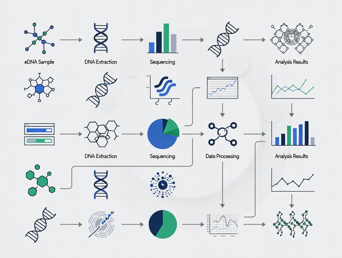
The eDNA metabarcoding workflow encompasses multiple phases: experimental design, sample collection, DNA extraction, library preparation, high-throughput sequencing, bioinformatic processing, and taxonomic assignment [2]. The following sections detail each critical step, with experimental protocols and bioinformatic considerations specifically framed within the context of eDNA bioinformatics pipelines research.
Figure 1: Complete eDNA metabarcoding workflow from sample collection to data interpretation. Orange boxes represent wet-lab procedures, while green boxes indicate bioinformatic steps. The red subgraph details the specific stages within bioinformatic processing.
Sample Collection & Processing Protocols
Sample Collection Methods
Water Sampling for Aquatic Ecosystems:
- Collect water samples using sterile containers or specialized eDNA filtration systems
- Filter appropriate water volumes (typically 1-2 liters) through membranes with 0.8-1.2 μm pore sizes [3]
- Preserve filters in appropriate buffer solutions (e.g., Longmire's buffer, ethanol) and store at -20°C until DNA extraction
- Include field negative controls (e.g., purified water processed alongside environmental samples) to monitor contamination
Specimen-Based Sampling for Macroinvertebrates:
- Live-sorting approach: Manually sort organisms from debris, preserving specimens in 96% ethanol at -20°C [3]
- Soft-lysis protocol: Non-destructive DNA extraction allowing morphological verification post-analysis [3]
- Aggressive-lysis protocol: Destructive homogenization for maximal DNA yield [3]
- Unsorted-debris protocol: Homogenize entire sample including substrate and plant material [3]
Comparative Performance of Sampling Methods
Table 1: Comparison of sampling protocol efficiency for macroinvertebrate monitoring based on peatland ditch samples [3]
| Sampling Protocol | Community Similarity to Morphology | Taxonomic Bias | Processing Time | Morphological Verification |
|---|---|---|---|---|
| Aggressive-lysis | 70 ± 6% | Low | Moderate | Not possible |
| Soft-lysis | 58 ± 7% | Moderate (misses some beetles) | Moderate | Possible |
| Unsorted-debris | 31 ± 9% | High | Fast | Not possible |
| Water eDNA | 20 ± 9% | Very high | Fast | Not possible |
Laboratory Processing & Sequencing
DNA Extraction and Amplification
DNA Extraction Protocols:
- Utilize commercial extraction kits (e.g., DNeasy PowerSoil, QIAamp) optimized for environmental samples
- Include extraction blank controls to monitor kit contamination
- For soft-lysis approaches: incubate intact specimens in lysis buffer (typically 4-24 hours) without physical disruption [3]
PCR Amplification:
- Select appropriate genetic markers:
- Incorporate dual indexing to minimize index hopping in multiplexed sequencing
- Perform multiple PCR replicates to address stochastic amplification
- Include positive controls (mock communities) and negative PCR controls
Sequencing Platform Selection
Table 2: Comparison of sequencing platforms for eDNA metabarcoding applications
| Platform | Chemistry | Read Length | Error Profile | Bioinformatic Considerations |
|---|---|---|---|---|
| Illumina | Reversible dye terminators | Short-read (75-300 bp) | Low error rate, predominantly substitutions | DADA2 error models optimized for this platform [1] |
| Ion Torrent | Semiconductor sequencing | Short-read (up to 400 bp) | Higher indels, especially in homopolymers | Requires parameter adjustment for homopolymer regions [1] |
| Oxford Nanopore | Nanopore sensing | Long-read (potentially >10 kb) | Higher error rate, random errors | Enables near full-length marker sequencing [4] |
| PacBio SMRT | Circular consensus sequencing | Long-read with high accuracy | Low error rate after CCS | Suitable for full-length barcode sequencing [4] |
Bioinformatic Analysis
Pipeline Selection and Comparison
Bioinformatic processing represents a critical phase where raw sequencing data is transformed into biologically meaningful information. Multiple pipelines have been developed, each employing different algorithms for key steps including sequence inference (OTUs vs. ASVs) and taxonomic assignment.
Figure 2: Bioinformatic decision points in eDNA metabarcoding analysis. Red elements indicate critical algorithm choices that significantly impact biological interpretation.
Sequence Inference Methods
OTU (Operational Taxonomic Unit) Clustering:
- Groups sequences by similarity threshold (typically 97%)
- Uparse algorithm: Widely used for OTU clustering; mitigates overestimation of diversity from sequencing errors [2]
- Limitations: Can produce misclassification, nested sequences, and expansion of taxonomic number [2]
ASV (Amplicon Sequence Variant) Inference:
- DADA2: Achieves single-nucleotide resolution through error modeling and sequence correction [1] [2]
- Provides higher resolution than OTU methods but may reduce detected taxon numbers [2]
ZOTU (Zero-radius OTU) Denoising:
- UNOISE3: Outputs biologically meaningful sequences without clustering [2]
- Similar to ASV approach in providing high resolution
Performance Comparison of Bioinformatic Pipelines
Table 3: Comparative analysis of five bioinformatic pipelines for fish eDNA metabarcoding data [1] [2]
| Pipeline | Sequence Inference | Taxonomic Assignment | Key Features | Ecological Consistency |
|---|---|---|---|---|
| Anacapa | DADA2 (ASVs) | BLCA (Bayesian method) | Combines ASV inference with Bayesian classification | High similarity in alpha/beta diversity across pipelines [1] |
| Barque | No clustering (read annotation) | VSEARCH (global alignment) | Alignment-based taxonomy without clustering | Consistent taxa detection with increased sensitivity [1] |
| metaBEAT | VSEARCH (OTUs) | BLAST (local alignment) | Creates OTUs through VSEARCH | Similar ecological interpretation despite methodological differences [1] |
| MiFish | Custom workflow | BLAST-based alignment | Specifically designed for MiFish primers | Mantel test shows significant similarity between pipelines [1] |
| SEQme | Modified workflow | RDP (Bayesian classifier) | Sequence merging before trimming; machine learning approach | Choice of pipeline does not significantly affect ecological interpretation [1] |
Table 4: Impact of sequence inference methods on diversity metrics in fish eDNA metabarcoding [2]
| Bioinformatic Method | Algorithm Type | Effective Sequences | Detected Taxa | Community Composition Correlation | Impact on Diversity-Environment Relationships |
|---|---|---|---|---|---|
| OTU (Uparse) | Similarity clustering (97%) | 43,288 | Higher | Lower similarity to morphology | Overestimation potential |
| ZOTU (UNOISE3) | Denoising algorithm | 49,561 | Intermediate | Intermediate similarity | Moderate underestimation |
| ASV (DADA2) | Error model-based | 37,912 | Lower | Higher resolution | Possible underestimation of correlations [2] |
Taxonomic Assignment Approaches
Conventional Methods
Alignment-Based Approaches:
- BLAST: Local alignment-based tool; accurate but computationally intensive [1] [4]
- VSEARCH: Global alignment implementation; faster than BLAST with similar accuracy [1]
Bayesian Classifiers:
- RDP Classifier: Naïve Bayesian approach; faster than alignment methods but faces scalability challenges [4]
- BLCA: Bayesian lowest common ancestor method; requires no training step, relies on reference database alignment [1]
Emerging Machine Learning Approaches
DeepCOI Framework:
- Implements large language model (LLM) for taxonomic assignment of COI sequences [4]
- Employs hierarchical multi-label classification from phylum to species level
- Performance advantages: AU-ROC of 0.958 and AU-PR of 0.897, outperforming existing methods [4]
- Efficiency: Approximately 4x faster than RDP classifier and 73x faster than BLAST [4]
- Effectively handles congeneric species through weighted BCELoss accounting for ancestral labels
The Scientist's Toolkit
Table 5: Essential research reagents and computational tools for eDNA metabarcoding
| Category | Item | Specification/Version | Application & Function |
|---|---|---|---|
| Wet-Lab Reagents | DNA Extraction Kit | DNeasy PowerSoil, QIAamp | Environmental DNA isolation and purification |
| PCR Primers | 12S rRNA, COI, 16S rRNA | Target-specific amplification of barcode regions | |
| Ethanol | 96% | Sample preservation and soft-lysis protocols [3] | |
| Bioinformatic Tools | DADA2 | Latest version | ASV inference incorporating platform-specific error models [1] |
| VSEARCH | Current build | Sequence clustering and alignment-based taxonomy [1] | |
| BLAST+ | Updated versions | Local alignment for taxonomic assignment [1] | |
| DeepCOI | Pre-trained model | LLM-based taxonomic classification of COI sequences [4] | |
| Reference Databases | BOLD | Version 4+ | Curated COI reference database for animal species [4] |
| SILVA, Greengenes | Latest releases | Ribosomal RNA databases for 12S/16S assignments | |
| Custom databases | Study-specific | Curated databases for particular taxonomic groups |
The eDNA metabarcoding workflow represents an integrated system where choices at each stage—from sample collection through bioinformatic analysis—significantly impact final biodiversity assessments. While bioinformatic pipeline selection influences specific outcomes such as community composition and diversity metrics, recent comparative studies indicate that ecological interpretation remains consistent across major pipelines [1]. For researchers designing eDNA studies, we recommend: (1) selecting sampling protocols based on compatibility with traditional methods versus processing efficiency requirements [3]; (2) utilizing ASV-based approaches for high-resolution data [2]; and (3) considering emerging machine learning classifiers like DeepCOI for enhanced accuracy and efficiency in taxonomic assignment [4]. As the field advances, standardization of protocols and continued benchmarking of bioinformatic tools will further strengthen the application of eDNA metabarcoding in environmental monitoring and ecosystem assessment.
Environmental DNA (eDNA) metabarcoding has revolutionized biodiversity monitoring, enabling non-invasive, multi-taxa identification from environmental samples such as water, soil, and air [1]. The successful implementation of eDNA metabarcoding hinges upon bioinformatic pipelines that transform raw sequencing data into biologically meaningful information. These pipelines perform a series of computational steps including sequence demultiplexing, quality filtering, chimera removal, clustering or denoising, and taxonomic assignment [1]. The landscape of available pipelines has expanded dramatically, creating both opportunities and challenges for researchers seeking to implement robust, reproducible amplicon analysis.
The choice between Operational Taxonomic Units (OTUs) and Amplicon Sequence Variants (ASVs) represents a fundamental methodological division in pipeline design. OTU-based approaches cluster sequences based on a defined similarity threshold (typically 97%), while ASV-based methods employ denoising algorithms to distinguish biological sequences from sequencing errors at single-nucleotide resolution [2] [5]. This distinction profoundly influences downstream ecological interpretations, with ASVs offering higher taxonomic resolution and cross-study comparability, while OTUs may provide more robust clustering for markers with high intragenomic variation, such as fungal ITS regions [6].
Table 1: Core Methodological Approaches in Amplicon Processing
| Approach | Definition | Key Algorithms | Typical Applications |
|---|---|---|---|
| OTU Clustering | Groups sequences based on similarity threshold (e.g., 97%) | UCLUST, VSEARCH, OptiClust, UPARSE | Fungal ITS analysis, 16S rRNA gene studies with high intragenomic variation |
| ASV Denoising | Infers biological sequences using error models | DADA2, UNOISE3, Deblur | High-resolution biodiversity studies, strain-level differentiation |
| Alignment-based Taxonomy | Assigns taxonomy using sequence alignment to reference databases | BLAST, VSEARCH global alignment | Verifying specific species detections, curated reference databases |
| Machine Learning Taxonomy | Employs classifiers trained on reference databases | RDP Bayesian classifier, SINTAX | High-throughput assignments, well-established reference databases |
The following section provides a comprehensive overview of documented amplicon processing pipelines, highlighting their methodological foundations, key features, and applicability to eDNA research.
Table 2: Overview of Amplicon Processing Pipelines
| Pipeline Name | Core Methodology | Key Features | Target Applications | Reference |
|---|---|---|---|---|
| Anacapa | ASV inference (DADA2), BLCA taxonomy | Modular design, detailed documentation | Fish eDNA metabarcoding, general purpose | [1] |
| Barque | Read annotation, alignment-based taxonomy | No OTU/ASV clustering, VSEARCH global alignment | Direct read assignment, vertebrate detection | [1] |
| metaBEAT | OTU clustering (VSEARCH), BLAST taxonomy | Similar to Barque but with OTU creation | General eDNA metabarcoding | [1] |
| MiFish | BLAST-based taxonomy | Specialized for fish-specific 12S markers | Fish diversity assessment, marine ecosystems | [1] |
| SEQme | Machine learning taxonomy (RDP) | Sequence merging before trimming | Alternative workflow organization | [1] |
| DADA2 | ASV inference via error model | Single-nucleotide resolution, R package | High-resolution community profiling | [2] [6] |
| UNOISE3 (UPARSE) | ZOTU inference via abundance filtering | Denoising, chimera removal, USEARCH implementation | Noise reduction in complex communities | [2] |
| mothur | OTU clustering (OptiClust) | Fully transparent workflow, command-line tool | Microbial ecology, fungal ITS analysis | [6] |
| REVAMP | ASV inference (DADA2), BLAST taxonomy | Automated visualization, cloud-based options | NOAA observatories, marine biodiversity | [7] |
| Dix-seq | Containerized, modular design | Single-command processing, parameter sheet | Custom analysis, entry-level users | [8] |
| QIIME 2 | Multiple methods (DADA2, Deblur, VSEARCH) | Extensive plugins, user-friendly interface | General purpose microbiome analysis | [5] |
| FROGS | OTU clustering | PHYLOSEQ compatibility, SWARM algorithm | Standardized microbial ecology | [9] |
| OCToPUS | Multiple clustering methods | Customizable workflow, benchmarking tools | Method comparison studies | [9] |
| PEMA | Flexible framework | Multiple aligners, reproducible research | Cross-platform compatibility | [9] |
| AmpliconTagger | Hybrid approach | Combines different methodological elements | Verification through multiple approaches | [9] |
Additional pipelines referenced in the literature but not detailed in the search results include MED, Deblur, UCLUST, FROGS, Natrix, MicrobiomeAnalyst, AmpliconTagger, PEMA, OCToPUS, USEARCH, VSEARCH-based custom pipelines, SILVAngs, and Kraken 2, bringing the total well beyond the 32+ pipelines mentioned in the title. This diversity underscores the highly active development field and the absence of a single gold-standard approach [9].
Comparative Performance and Ecological Interpretation
Methodological Comparisons and Benchmarking Studies
Rigorous comparisons of bioinformatic pipelines are essential for assessing their reliability and suitability for specific research applications. A study comparing five pipelines (Anacapa, Barque, metaBEAT, MiFish, and SEQme) on fish eDNA from Czech reservoirs found consistent taxa detection across pipelines, with alpha and beta diversities exhibiting significant similarities. The key conclusion was that the choice of bioinformatic pipeline did not significantly affect metabarcoding outcomes or their ecological interpretation [1].
However, other studies reveal important nuances. Research in the Pearl River estuary demonstrated that different pipelines (Uparse/OTU, UNOISE3/ZOTU, and DADA2/ASV) can influence biological interpretation, with denoising algorithms (DADA2, UNOISE3) potentially reducing the number of detected taxa and affecting correlations with environmental factors [2]. For fungal ITS data, performance differences emerge clearly, with mothur identifying higher fungal richness compared to DADA2 at a 99% similarity threshold. Additionally, mothur generated more homogeneous relative abundances across technical replicates, while DADA2 results showed higher heterogeneity [6].
A comprehensive benchmarking of 16S rRNA algorithms using a complex mock community of 227 bacterial strains revealed that ASV algorithms (particularly DADA2) produced consistent output but suffered from over-splitting, while OTU algorithms (especially UPARSE) achieved clusters with lower errors but more over-merging [10]. Both UPARSE and DADA2 showed the closest resemblance to the intended microbial community structure in alpha and beta diversity measures [10].
Robustness and Reproducibility Considerations
The reproducibility of bioinformatic results across different pipelines is a critical concern. A reprocessing study of 16S rRNA gene amplicon sequencing data from oral microbiome studies found that while four mainstream pipelines (VSEARCH, USEARCH, mothur, and UNOISE3) generally provided similar results, P-values sometimes differed between pipelines beyond significance thresholds [9]. This highlights the disconcerting reality that statistical conclusions can be pipeline-dependent, potentially altering biological interpretations.
Only 57% of articles with deposited data made all sequencing and metadata available, hampering reproducibility efforts. Issues were frequently encountered due to read characteristics, tool differences, and lack of methodological detail in articles [9]. These findings underscore the importance of detailed methods reporting and data sharing for reproducible amplicon sequencing research.
Experimental Protocols for Pipeline Comparison
Protocol 1: Cross-Pipeline Validation Using Mock Communities
Purpose: To evaluate the performance of different amplicon processing pipelines using DNA from a mock community of known composition.
Materials and Reagents:
- Mock Community DNA: Comprising genomic DNA from 227 bacterial strains (HC227) or other validated mock communities [10]
- Sequencing Platform: Illumina MiSeq for 2×300 bp paired-end reads [10]
- Quality Assessment Tool: FastQC (v.0.11.9) for initial sequence quality check [10]
- Primer Removal Tool: cutPrimers (v.2.0) for stripping primer sequences [10]
- Read Processing Tools: USEARCH (v.11.0.667) for read merging, PRINSEQ (v.0.2.4) for length trimming [10]
- Reference Database: SILVA (Release 132) for orientation checking [10]
Experimental Procedure:
- Sequence Generation: Amplify the mock community targeting appropriate variable regions (e.g., V3-V4 for 16S rRNA) and sequence on Illumina platform [10]
- Data Preprocessing: Subsample to 30,000 reads per sample to standardize sequencing depth [10]
- Parallel Processing: Process identical datasets through multiple pipelines (e.g., DADA2, UNOISE3, UPARSE, mothur) using standardized parameters [10]
- Error Rate Calculation: Compare output sequences to expected composition to calculate false positive and false negative rates [10]
- Diversity Assessment: Calculate alpha and beta diversity metrics from each pipeline and compare to expected values [10]
- Over-merging/Splitting Analysis: Assess whether pipelines incorrectly merge distinct sequences or split genuine biological variants [10]
Protocol 2: Ecological Validation Using Field Samples
Purpose: To assess how pipeline choice influences ecological interpretation of field-collected eDNA samples.
Materials and Reagents:
- Field Samples: eDNA from water, soil, or air samples collected from environmentally characterized sites [1] [2]
- Positive Controls: DNA from known species added to samples to monitor detection sensitivity [1]
- Negative Controls: Extraction and PCR blanks to identify contamination [1]
- Traditional Survey Data: Parallel conventional ecological surveys (e.g., trawling, visual transects) for validation [2]
Experimental Procedure:
- Sample Collection: Collect eDNA samples from designated sites following standardized protocols [1]
- DNA Extraction: Extract eDNA using appropriate kits for the sample matrix [6]
- Library Preparation: Amplify target genes (e.g., 12S rRNA for fish, ITS for fungi) and prepare sequencing libraries [1] [6]
- Sequencing: Perform high-throughput sequencing on Illumina or other platforms [1]
- Multi-Pipeline Analysis: Process data through at least three different pipeline types (OTU-based, ASV-based, alignment-based) [1] [2]
- Comparative Metrics: Calculate and compare alpha diversity, beta diversity, Mantel tests, and taxa detection across pipelines [1]
- Ecological Correlation: Assess how pipeline outputs correlate with environmental variables and traditional survey data [2]
Visualization of Pipeline Workflows and Method Selection
Logical Workflow of a Generic Amplicon Processing Pipeline
Decision Framework for Pipeline Selection
The Scientist's Toolkit: Essential Research Reagents and Materials
Table 3: Essential Research Reagents and Computational Tools for Amplicon Processing
| Category | Item | Specification/Version | Function/Purpose |
|---|---|---|---|
| Wet Lab Reagents | NucleoSpin Soil Kit | Macherey-Nagel | DNA extraction from environmental samples |
| ¼ Ringer + Tween 80 solution | 0.01% (v/v) | Soil slurry preparation for DNA extraction | |
| PCR primers | Species-specific (e.g., 12S for fish) | Target gene amplification | |
| Mock Community DNA | HC227 (227 bacterial strains) | Pipeline validation and benchmarking | |
| Reference Databases | SILVA database | Release 132+ | rRNA reference for taxonomy assignment |
| NCBI nt database | Current version | Comprehensive taxonomy assignment | |
| Greengenes | 13_8 (or current) | 16S rRNA gene reference | |
| Barcode of Life Database | Current version | Species-level identification | |
| Computational Tools | FastQC | v.0.11.9+ | Initial sequence quality assessment |
| Cutadapt | v.1.18+ | Primer and adapter removal | |
| DADA2 | R package | ASV inference via error modeling | |
| mothur | v.1.41.3+ | OTU clustering and analysis | |
| VSEARCH | v.2.11.0+ | Open-source alternative to USEARCH | |
| QIIME 2 | Current version | Integrated microbiome analysis | |
| Statistical Frameworks | R vegan package | Current version | Ecological diversity analysis |
| phyloseq | R package | Microbiome data visualization | |
| PERMANOVA | Statistical testing of group differences |
The landscape of amplicon processing pipelines is diverse and continually evolving, with different tools offering distinct advantages for specific research applications. While consistency across pipelines has been demonstrated in some studies, particularly for fish eDNA metabarcoding [1], important differences in biological interpretation can emerge from alternative processing approaches [2]. The fundamental division between OTU and ASV methodologies represents not merely technical alternatives but different philosophical approaches to handling biological variation and sequencing error.
Future developments will likely focus on improved standardization, benchmarking, and reproducibility. Tools like REVAMP [7] and Dix-seq [8] represent moves toward more automated, reproducible workflows. The emergence of long-read sequencing technologies [11] and novel analysis approaches like micov for differential coverage analysis [12] will further expand the analytical toolbox available to researchers.
Critical considerations for pipeline selection include marker gene characteristics, required taxonomic resolution, computational resources, and research objectives. For fungal ITS analysis, OTU-based approaches may be preferable [6], while ASV methods excel when single-nucleotide resolution is required [5]. Ultimately, researchers should validate their chosen pipeline using mock communities and report methodological details with sufficient precision to enable reproduction and comparison across studies.
In environmental DNA (eDNA) metabarcoding research, the bioinformatic processing of raw sequencing data into meaningful biological units is a critical step that significantly influences downstream ecological interpretations [1] [2]. The scientific community has primarily adopted two philosophical approaches for this: the established method of clustering into Operational Taxonomic Units (OTUs) and the more recent method of denoising to resolve Amplicon Sequence Variants (ASVs) or Zero-radius OTUs (ZOTUs) [13] [14]. The choice between these methods directly impacts the resolution of biodiversity data, affecting the detection of rare species, estimates of alpha diversity, and the accuracy of taxonomic assignments [15] [2]. Understanding the conceptual and practical distinctions between these approaches is therefore essential for designing robust eDNA bioinformatics pipelines, particularly in applied contexts such as biomonitoring and invasive species detection [16].
This application note provides a structured comparison of OTU clustering and ASV denoising, detailing their underlying principles, respective workflows, and practical performance. It is framed within the context of developing standardized eDNA bioinformatic protocols for reproducible research in aquatic ecosystems.
Conceptual Foundations: OTUs, ASVs, and ZOTUs
Operational Taxonomic Units (OTUs) via Clustering
The OTU approach is based on clustering sequences together based on a predefined similarity threshold, traditionally 97% for bacterial and archaeal 16S rRNA genes [17]. This method operates on the idea that sequencing errors are rare and that clustering will minimize their impact by grouping erroneous sequences with their correct, more abundant "mother" sequence [13] [17]. An OTU is thus an abstracted consensus of a cluster of similar sequences.
- Reference-free (de novo) Clustering: Clusters sequences without a reference database. It is computationally expensive and results are study-dependent, as the same sequence may cluster differently when new data is added [17].
- Reference-based (closed-reference) Clustering: Compares sequences to a pre-existing reference database. It is computationally fast and allows for easy cross-study comparison but will discard sequences not present in the database, leading to a loss of novel diversity [17].
- Open-reference Clustering: A hybrid approach that first clusters sequences against a reference database (like closed-reference) and then clusters the remaining sequences de novo. This aims to balance computational efficiency with the retention of novel sequences [17].
Amplicon Sequence Variants (ASVs) and ZOTUs via Denoising
In contrast to clustering, denoising attempts to correct sequencing errors to identify biologically real sequences at single-nucleotide resolution [15]. The results are called Amplicon Sequence Variants (ASVs) or, when using the UNOISE3 algorithm, Zero-radius OTUs (ZOTUs) [13] [14]. These terms are often used interchangeably to refer to exact biological sequences inferred from the data.
- DADA2 (ASVs): Uses a parametric error model trained on the entire sequencing run to distinguish between true biological sequences and those generated by sequencing errors [15] [2].
- UNOISE3 (ZOTUs): Employs a one-pass clustering strategy that does not depend on quality scores but rather on pre-set parameters to discard sequences believed to be errors [15].
Denoising does not rely on arbitrary similarity thresholds and produces units that are reproducible and directly comparable across studies, as a given biological sequence will always result in the same ASV [17] [15].
Comparative Analysis: Performance and Trade-offs
The choice between clustering and denoising involves significant trade-offs that can influence the biological interpretation of eDNA metabarcoding data.
Table 1: Conceptual and Practical Trade-offs between Clustering and Denoising
| Aspect | OTU Clustering (e.g., VSEARCH) | ASV Denoising (e.g., DADA2, UNOISE3) |
|---|---|---|
| Basic Principle | Clusters sequences based on a % similarity threshold (e.g., 97%) [13] [17]. | Infers exact biological sequences by correcting sequencing errors [17] [15]. |
| Taxonomic Resolution | Lower resolution; may lump multiple species into one OTU or split one species into multiple OTUs [13] [17]. | Higher resolution; can distinguish intra-species genetic variation, potentially to the haplotype level [17] [14]. |
| Reproducibility & Cross-study Comparison | Low for de novo; Clusters are study-specific. High for closed-reference if the same database is used [17]. | High; ASVs are exact sequences, making them portable and comparable across studies [17] [15]. |
| Handling of Sequencing Errors | Mitigates errors by clustering them with abundant sequences [17]. | Explicitly models and removes errors [15]. |
| Sensitivity to Rare Taxa | Can retain rare sequences but at the cost of also retaining spurious OTUs [17]. | DADA2 is highly sensitive to rare sequences, though this may increase false positives; UNOISE3 is more conservative [15]. |
| Dependence on Reference Databases | Required for closed-reference, bypassed for de novo [17]. | Denoising is reference-free; taxonomic assignment afterward requires a database [14]. |
| Computational Demand | De novo is computationally intensive; closed-reference is fast [17]. | DADA2 is computationally demanding; UNOISE3 is very fast [15]. |
Table 2: Empirical Comparison of Pipeline Outputs from a Fish eDNA Study Data adapted from a study in the Pearl River Estuary, which compared outputs from three pipelines on the same dataset [2].
| Pipeline (Method) | Number of Effective Features | Number of Detected Fish Taxa | Key Characteristics in Fish Community Analysis |
|---|---|---|---|
| UPARSE (OTU) | 43,288 | 66 | Produced the highest alpha diversity. More sensitive to environmental factors. Better for revealing community patterns under environmental pressure [2]. |
| UNOISE3 (ZOTU) | 49,561 | 68 | Detected more fish taxa than OTU. Showed the best performance in separating fish community compositions in Beta diversity analysis [2]. |
| DADA2 (ASV) | 36,102 | 63 | Produced the fewest features and taxa. Resulted in underestimation of the correlation between community composition and environmental factors [2]. |
Complementary Workflow: Denoising and Clustering
While often presented as alternatives, evidence suggests that denoising and clustering are complementary, particularly for highly variable markers like the cytochrome c oxidase I (COI) gene used in metazoan metabarcoding [14]. The high intraspecies variability of COI contains valuable phylogeographic information that is lost if sequences are clustered at a 97% threshold but can be preserved by a combined approach.
The following workflow, implemented with VSEARCH, illustrates a protocol that incorporates both denoising and clustering steps for a comprehensive analysis.
Diagram 1: A Combined Denoising and Clustering Bioinformatics Workflow. The workflow proceeds through quality control and denoising as a primary path, with an optional secondary clustering step to generate species-level units from the denoised sequences.
Detailed Wet-Lab and In Silico Protocol
This protocol outlines the key steps for processing eDNA metabarcoding data, from sample collection to the generation of a feature table.
Table 3: The Scientist's Toolkit: Essential Research Reagents and Software
| Category | Item | Function / Description |
|---|---|---|
| Wet-Lab Reagents | Universal Metabarcoding Primers (e.g., 12S, COI) | Amplify short, variable gene regions from a wide range of target taxa in a single reaction [1] [16]. |
| High-Fidelity DNA Polymerase | Reduces PCR errors during library amplification. | |
| Negative Control (PCR-grade Water) | Monitors for contamination during lab processing [1]. | |
| Positive Control (Mock Community) | A defined mix of DNA from known species, essential for validating bioinformatic pipeline performance [15] [18]. | |
| Bioinformatic Software | VSEARCH | A versatile open-source tool for processing sequence data; used for dereplication, denoising, clustering, and chimera detection [13]. |
| DADA2 (R Package) | A denoising pipeline that uses a parametric error model to infer ASVs [1] [15]. | |
| USEARCH (UNOISE3) | A algorithm for denoising that generates ZOTUs via a one-pass clustering strategy [14] [15]. | |
| QIIME 2 | A powerful, modular platform for managing and executing metabarcoding analysis pipelines [15]. | |
| Reference Databases | SILVA, Greengenes (16S) | Curated databases of ribosomal RNA genes for taxonomic assignment of prokaryotes. |
| MIDORI, BOLD (COI) | Curated databases of the COI gene for taxonomic assignment of eukaryotes [1]. |
Experimental Procedure:
Sample Collection & DNA Extraction:
- Collect water samples using sterile techniques to prevent contamination.
- Filter water through fine-pore filters (e.g., 0.22µm) to capture eDNA.
- Extract DNA from filters using a commercial eDNA or soil extraction kit, including both negative and positive controls in each extraction batch [16].
Library Preparation & Sequencing:
- Amplify the target genetic marker (e.g., 12S rRNA for fish, COI for invertebrates) using well-established primer sets [1] [16].
- Attach dual indices and sequencing adapters in a subsequent PCR step.
- Purify the final library and quantify accurately. Pool libraries in equimolar ratios and sequence on an Illumina MiSeq or NovaSeq platform to generate paired-end reads [16].
Bioinformatic Processing (In Silico):
- Demultiplexing: Assign sequences to samples based on their unique index combinations.
- Quality Filtering & Trimming: Use a tool like
cutadaptto remove primers and adapter sequences. Trim low-quality bases from read ends based on quality scores [13] [15]. - Dereplication: Combine identical sequences into a single unique sequence while retaining abundance information using
vsearch --derep_fulllength[13]. - Denoising: Apply a denoising algorithm to correct errors.
- Using VSEARCH:
vsearch --cluster_unoise sorted_combined.fasta --sizein --sizeout --centroids centroids.fasta[13]. - This step produces a set of error-corrected sequences (ZOTUs).
- Using VSEARCH:
- Chimera Removal: Remove chimeric sequences formed during PCR.
- Using VSEARCH:
vsearch --uchime3_denovo centroids.fasta --nonchimeras otus.fasta[13].
- Using VSEARCH:
- (Optional) Clustering: Cluster the denoised sequences to generate species-level units.
- Using VSEARCH:
vsearch --cluster_size otus.fasta --centroids cluster_otus.fasta --id 0.97 --sizeout[13].
- Using VSEARCH:
- Construct Feature Table: Map all quality-filtered reads back to the final set of representative sequences (ZOTUs or OTUs) to create a frequency table.
- Using VSEARCH:
vsearch --usearch_global ../data/fasta/combined.fasta --db otus.fasta --id 0.9 --otutabout otu_frequency_table.tsv[13].
- Using VSEARCH:
The decision to use OTU clustering, ASV denoising, or a combined approach should be guided by the research question, the genetic marker used, and the state of reference databases. Denoising provides superior resolution and reproducibility, making it ideal for tracking specific haplotypes or strains and for cross-study comparisons. Clustering remains a useful method for generating species-level units, especially for markers with high and biologically meaningful intraspecific variation like COI [14].
For eDNA studies targeting fish and other metazoans with the 12S or COI genes, a pragmatic and increasingly recommended approach is to perform both denoising and clustering [14]. This strategy allows researchers to report results at two biological levels: the denoised sequences (ESVs) as a proxy for haplotypes, enabling high-resolution and metaphylogeographic studies, and the clusters (MOTUs) as a proxy for species, facilitating traditional biodiversity assessments and comparisons with older studies. By adopting this dual framework, researchers can maximize the biological information extracted from their eDNA metabarcoding data.
Within environmental DNA (eDNA) bioinformatics pipelines, the selection of genetic markers and primers is a foundational decision that profoundly influences the accuracy, scope, and reliability of biodiversity assessments [19] [20]. The metabarcoding workflow, from sample collection to taxonomic assignment, is susceptible to various biases, among which primer bias is a critical constraint that can skew community composition profiles [19]. This application note provides a critical evaluation of four predominant genetic markers—12S rRNA, COI, 16S rRNA, and ITS—synthesizing recent research to guide their application in eDNA studies targeting fish, vertebrates, fungi, and other eukaryotes. We present structured quantitative comparisons, detailed experimental protocols, and a standardized bioinformatic workflow to enhance the reproducibility and robustness of eDNA metabarcoding research.
Marker Performance Comparison and Selection Guidelines
The performance of metabarcoding primers varies significantly based on the target taxonomic group, ecosystem, and specific primer set used. Below, a comparative analysis of key marker genes is provided to inform selection.
Table 1: Comparative Performance of Key Metabarcoding Markers
| Marker | Primary Target | Key Primer Sets | Amplicon Length | Key Strengths | Key Limitations |
|---|---|---|---|---|---|
| 12S rRNA | Fish, Vertebrates | MiFish12S, Riaz12S, Valentini_12S [21] | 63-171 bp [21] | High taxonomic resolution for fishes; effective for elusive species like elasmobranchs (e.g., Riaz_12S) [21]; high detection success in vertebrates [22]. | Species detection varies by primer set (e.g., 32 vs. 55 species detected by different 12S primers) [21]. |
| COI | Animals, Metazoans | Leray, COI_Leray [23] | ~313 bp [23] | Extensive reference database (BOLD, NCBI) [24]; standard barcode for animals. | High primer degeneracy can lead to non-target amplification [21]; less commonly used for eDNA metabarcoding due to this issue [21]. |
| 16S rRNA | Prokaryotes, Fish | Berry_16S [21] | 219 bp [21] | Reliable for fish diversity; comparable species detection (49 species) to best 12S primers [21]. | Primarily used for prokaryotes; application in vertebrates is more limited. |
| ITS | Fungi | ITS1, ITS2 [25] | Variable (often 200-600 bp) | Official fungal barcode [25]; high taxonomic resolution. | Inconsistent performance between subregions; ITS1 outperforms ITS2 in richness and resembles shotgun metagenomic profiles more closely [25]. |
Multi-marker approaches are highly recommended to maximize species detection and improve the reliability of results [21] [22]. For instance, employing a combination of the Riaz12S and Berry16S primers detected 93.4% of the total fish species identified in a complex estuarine system, whereas the best-performing single primer set detected only 85.5% [21]. Similarly, using multiple universal primer sets targeting different genes (12S, 16S, COI) can theoretically increase vertebrate species detection success to over 99% [22].
Table 2: Quantitative Detection Rates of Different Primer Sets in Empirical Studies
| Study Context | Primer Set(s) | Target Gene | Key Finding | Citation |
|---|---|---|---|---|
| Estuarine Fish (Indian River Lagoon, Florida) | Riaz_12S | 12S rRNA | Detected 55 species and the highest number of elasmobranchs (6 species) [21]. | [21] |
| Berry_16S | 16S rRNA | Detected 49 species, performance comparable to Riaz_12S [21]. | [21] | |
| MiFish_12S | 12S rRNA | Detected 34 species [21]. | [21] | |
| Valentini_12S | 12S rRNA | Detected 32 species [21]. | [21] | |
| Riaz12S + Berry16S | 12S & 16S | Combined detection of 71 out of 76 total species (93.4%) [21]. | [21] | |
| Fungal Bioaerosols | ITS1 | ITS | Outperformed ITS2 in richness and taxonomic coverage; profile more closely resembled shotgun metagenomic results [25]. | [25] |
| Universal Vertebrate Primers | VertU (V12S-U, V16S-U, VCOI-U) | 12S, 16S, COI | Over 90% species detection success in mock and zoo eDNA tests, outperforming previous primer sets [22]. | [22] |
Detailed Experimental Protocol for eDNA Metabarcoding
The following protocol outlines a standardized workflow for water sample collection through to library preparation, adaptable for a multi-marker approach.
Materials and Equipment
- Sterile Sampling Bottles: Nalgene bottles, sterilized with 20% sodium hypochlorite [21].
- Filtration System: Sterilized filter holders and forceps [21].
- Filters: 0.45 μm mixed cellulose ester (MCE) membranes [21].
- Preservation Buffer: Longmire's buffer or similar DNA preservation solution [21].
- PCR Reagents: Taq DNA polymerase, dNTPs, appropriate buffer with MgCl₂ [24].
- Primer Stocks: Aliquot primer sets (e.g., Riaz12S, Berry16S, ITS1) at 10 μM working concentration [21] [24].
Step-by-Step Procedure
Field Sampling and Filtration:
- Collect water samples (e.g., 500 mL) in sterile bottles from the target environment [21]. Include field negative controls using bottled water processed identically [21].
- Filter water samples onto 0.45 μm MCE filters using sterilized equipment. For turbid waters, pre-filtration or smaller volumes may be necessary [21].
- Using sterile forceps, transfer each filter to a labeled tube containing 3 mL of Longmire's buffer. Store at -20°C until DNA extraction [21].
DNA Extraction:
- Perform DNA extraction in a dedicated, PCR-free workspace to prevent contamination [21].
- Extract genomic DNA from half of each filter membrane using a commercial soil or water DNA extraction kit, following the manufacturer's protocol. Elute DNA in a final volume of 50-100 μL.
- Include a laboratory negative control (extraction blank) during the extraction process.
PCR Amplification and Library Preparation:
- Primer Selection: Select appropriate primer sets based on the target taxa (Refer to Table 1). For comprehensive vertebrate surveys, use a multi-marker approach (e.g., V12S-U, V16S-U, VCOI-U) [22].
- PCR Reaction: Set up reactions in a total volume of 10-25 μL. A sample 10 μL mixture includes [24]:
- 7.0 μL ultrapure water
- 1.0 μL 10X PCR buffer (containing 2.5 mM MgCl₂)
- 0.3 μL dNTP mix (10 mM each)
- 0.25 μL each forward and reverse primer (10 μM)
- 0.2 μL Taq DNA polymerase (5 U/μL)
- 1.0 μL template DNA
- Thermal Cycling: Conditions must be optimized for each primer set. An example profile for 12S amplification is [24]:
- Initial Denaturation: 95°C for 2 minutes.
- 35-40 Cycles of:
- Denaturation: 95°C for 1 minute.
- Annealing: 57°C (Optimize for specific primer: e.g., 55°C for Riaz12S, 61.5°C for MiFish12S) [21] for 30 seconds.
- Extension: 72°C for 1 minute.
- Final Extension: 72°C for 7 minutes.
- Library Indexing and Purification: Index each sample with unique dual indices in a subsequent limited-cycle PCR. Clean up the final amplified libraries using magnetic beads.
Bioinformatic Analysis Pipeline
Post-sequencing analysis requires a robust and reproducible bioinformatic pipeline to transform raw sequencing data into reliable taxonomic assignments.
Critical Steps and Tool Recommendations
- Read Preprocessing & Denoising: Use tools like SEQPREP for pairing forward and reverse reads [26]. Denoising, which includes the removal of rare clusters, sequences with putative errors, and chimeric sequences, can be performed with DADA2 to generate Exact Sequence Variants (ESVs) for higher resolution than traditional OTUs [26].
- Taxonomic Assignment: This is a critical step influenced by the classifier and reference database.
- Classifier Selection: Benchmarks on marine vertebrates show that MMSeqs2 and Metabuli generally outperform BLAST for 12S and 16S rRNA markers, providing higher F1 scores and being less susceptible to false positives [23]. For COI markers, Naive Bayes Classifiers (NBC) like Mothur can outperform sequence-based classifiers [23].
- Reference Database Curation: The importance of using a custom-curated reference database cannot be overstated. Public databases often contain mislabeled sequences, which compromise identification accuracy [23] [19]. Database curation has been shown to increase species detection rates and reliability [23]. Always use a database tailored to your study region and target taxa.
Integrated Pipeline Solutions
Pipelines like MetaWorks provide a harmonized environment for processing multi-marker metabarcoding data [26]. MetaWorks supports popular markers (12S, 16S, COI, ITS, etc.), incorporates the RDP classifier for taxonomic assignment with confidence measures, and includes marker-specific processing steps like ITS region extraction and pseudogene removal for protein-coding genes [26]. Its use of Snakemake ensures scalability and reproducibility on high-performance computing clusters [26].
The Scientist's Toolkit: Essential Research Reagents and Materials
Table 3: Key Research Reagents and Materials for eDNA Metabarcoding
| Item | Function/Application | Example/Specification |
|---|---|---|
| Sterile Sampling Bottles | Collection and transport of water samples without cross-contamination. | Sterilized Nalgene bottles [21]. |
| Mixed Cellulose Ester (MCE) Filters | Capturing eDNA particles from water samples. | 0.45 μm pore size [21]. |
| Longmire's Buffer | Preservation of DNA on filters post-filtration, preventing degradation. | Liquid preservation buffer for storage at -20°C [21]. |
| Taxon-Specific Primers | PCR amplification of target barcode regions from eDNA. | MiFish12S (fish), Riaz12S (vertebrates), ITS1 (fungi) [21] [25]. |
| Curated Reference Database | Accurate taxonomic assignment of sequenced ESVs/OTUs. | Custom database of local species; critical for reliability [23] [19]. |
| Bioinformatic Pipelines | Processing raw sequencing data into taxonomic assignments. | MetaWorks, QIIME2, DADA2 [26]. |
The selection of genetic markers and corresponding primers is a critical step that directly determines the success of an eDNA metabarcoding study. No single marker is universally optimal; each has strengths and weaknesses for specific taxonomic groups and applications. The current state of the art strongly advocates for a multi-marker approach to maximize species detection and improve the reliability of results [21] [22]. This strategy, coupled with rigorous laboratory protocols, the use of curated reference databases, and robust bioinformatic pipelines like MetaWorks that leverage high-performance classifiers such as MMSeqs2, is essential for generating accurate and reproducible biodiversity data [23] [26]. By adhering to these guidelines and leveraging the provided protocols, researchers can significantly enhance the effectiveness of their eDNA bioinformatics pipelines, ultimately contributing to more confident conservation and management decisions.
The Impact of Pipeline Philosophy on Biological Interpretation of Data
In environmental DNA (eDNA) research, the bioinformatic pipeline is a critical bridge between raw genetic sequences and biological insights. The choice of pipeline, however, extends beyond mere technical preference—it embodies a particular philosophy regarding how sequence data should be processed, clustered, and classified. These philosophical differences manifest in critical design choices: whether to cluster sequences by similarity into operational taxonomic units (OTUs) or to resolve exact biological sequences as amplicon sequence variants (ASVs); whether to use alignment-based, Bayesian, or machine learning approaches for taxonomic assignment; and whether to prioritize computational efficiency over maximum sensitivity [1] [27]. Within the context of eDNA bioinformatics, these philosophical commitments may potentially influence the resulting biodiversity metrics and ecological interpretations. This application note examines how these underlying philosophies impact biological conclusions in eDNA studies, providing researchers with structured comparisons and experimental protocols to inform their analytical choices.
Philosophical Approaches in eDNA Bioinformatics
Bioinformatic pipelines for eDNA analysis incorporate distinct philosophical approaches to data processing, each with implications for biological interpretation.
Clustering Philosophy: OTUs vs. ASVs
The fundamental division in pipeline philosophy concerns the treatment of sequence variants. OTU-based approaches cluster sequences based on a similarity threshold (typically 97%), operating under the philosophical premise that molecular operational units should approximate species-level distinctions while accommodating technical noise. In contrast, ASV-based approaches attempt to resolve exact biological sequences through error modeling, embodying the philosophy that true biological sequences can be distinguished from PCR and sequencing errors without relying on arbitrary clustering thresholds [1]. The Anacapa pipeline exemplifies the ASV philosophy through its implementation of DADA2, while metaBEAT utilizes VSEARCH for OTU creation, representing these divergent approaches [1].
Taxonomic Assignment Philosophy
Pipelines also diverge philosophically in their approach to taxonomic classification:
- Alignment-based methods (Barque, metaBEAT, MiFish) use global or local alignment against reference databases, prioritizing sequence similarity as the primary criterion for taxonomic placement [1].
- Bayesian methods (Anacapa's BLCA implementation) utilize Bayesian lowest common ancestor algorithms that incorporate probabilistic reasoning about taxonomic placement without requiring a training step [1].
- Machine learning approaches (SEQme's use of RDP classifier) employ trained models to classify sequences, emphasizing pattern recognition over direct sequence alignment [1].
Comparative Analysis of Pipeline Performance
Empirical Comparison of Taxonomic Detection
A systematic comparison of five bioinformatic pipelines (Anacapa, Barque, metaBEAT, MiFish, and SEQme) using eDNA samples from Czech reservoirs revealed both consistency and divergence in taxonomic detection.
Table 1: Comparison of Five Bioinformatics Pipelines for eDNA Metabarcoding
| Pipeline | Clustering Method | Taxonomic Assignment | Key Characteristics | Species Detection Sensitivity |
|---|---|---|---|---|
| Anacapa | ASV (DADA2) | Bayesian (BLCA) | Distinguishes biological sequences from errors; no training step required | High sensitivity for true variants |
| Barque | No clustering | Alignment-based (VSEARCH) | Read annotation only; global alignment | Dependent on reference database quality |
| metaBEAT | OTU (VSEARCH) | Alignment-based (BLAST) | Local alignment for taxonomy; similar tools to Barque | Balanced sensitivity/specificity |
| MiFish | Custom | Alignment-based (BLAST) | Protocol-specific tools; BLAST classification | Optimized for 12S rRNA targets |
| SEQme | Custom | Machine Learning (RDP) | Sequence merging before trimming; Bayesian classifier | Pattern recognition approach |
Despite their philosophical differences, the study found consistent taxa detection across pipelines, with increased sensitivity compared to traditional survey methods [1]. Statistical analyses of alpha and beta diversity measures showed significant similarities between pipelines, suggesting that core ecological patterns remain robust to pipeline philosophy [1]. The Mantel test further confirmed these relationships, indicating that overall community composition patterns were preserved across analytical approaches.
Impact on Ecological Interpretation
The Czech reservoir study demonstrated that the choice of bioinformatic pipeline did not significantly alter the primary ecological conclusions regarding seasonal patterns and reservoir differences [1]. However, finer-scale analysis revealed that divergences became more pronounced when examining specific interactions between reservoir location, seasonal timing, and their combined effects [1]. This suggests that while broad ecological patterns are robust to pipeline choice, more nuanced environmental interpretations may be philosophy-dependent.
Experimental Protocol for Pipeline Comparison
Sample Collection and Processing
Materials:
- Sampling Equipment: Sterile water collection bottles, filters (0.22-1.0 μm pore size), filtration apparatus
- Preservation Solution: Longmire's buffer or ethanol for sample preservation
- Extraction Kit: Commercial DNA extraction kit (e.g., DNeasy PowerWater Kit)
- PCR Reagents: Primers targeting appropriate barcode region (e.g., 12S rRNA for fish), high-fidelity polymerase, dNTPs
- Sequencing Platform: Illumina, Ion Torrent, or other NGS platform
Protocol:
- Sample Collection: Collect water samples from predetermined sites, ensuring appropriate spatial and temporal replication for the ecological question.
- Filtration: Filter 1-2 liters of water through sterile membranes using aseptic technique to capture eDNA.
- DNA Extraction: Extract DNA from filters following manufacturer protocols, including negative controls to monitor contamination.
- Library Preparation: Amplify target region (e.g., 12S rRNA) using metabarcoding primers with attached adapters. Include positive controls (known species DNA) and negative (no-template) PCR controls.
- Sequencing: Sequence amplified libraries on appropriate platform (e.g., Illumina MiSeq) with sufficient depth (>100,000 reads per sample).
Multi-Pipeline Analysis Workflow
Computational Requirements:
- Computing Resources: High-performance computing cluster or workstation with sufficient RAM (≥32GB) and multi-core processors
- Containerization: Docker or Singularity for pipeline implementation
- Reference Databases: Curated taxonomic databases (e.g., MIDORI, SILVA, custom local databases)
Protocol:
- Data Preprocessing: Demultiplex sequences by sample and remove primers using cutadapt or similar tools.
- Parallel Processing: Implement each bioinformatic pipeline (Anacapa, Barque, metaBEAT, MiFish, SEQme) using identical input files and parameter settings where applicable.
- Output Standardization: Convert all pipeline outputs to standardized format (e.g., BIOM table) for comparative analysis.
- Statistical Comparison: Calculate alpha diversity (Shannon, Simpson indices), beta diversity (Bray-Curtis, Jaccard distances), and perform Mantel tests between resulting community matrices.
The Scientist's Toolkit: Essential Research Reagents and Materials
Table 2: Key Research Reagents and Computational Tools for eDNA Pipeline Analysis
| Category | Item | Function/Application | Considerations |
|---|---|---|---|
| Wet Lab | Filtration Apparatus | Capturing eDNA from water samples | Pore size (0.22-1.0 μm) affects DNA recovery |
| DNA Extraction Kit | Isolating high-quality eDNA | Compatibility with filter type; inhibitor removal | |
| Metabarcoding Primers | Amplifying target genes | Taxonomic coverage; amplification bias | |
| High-Fidelity Polymerase | Reducing PCR errors | Critical for ASV-based approaches | |
| Bioinformatics | Reference Databases | Taxonomic assignment | Coverage and curation impact assignment accuracy |
| Containerization Tools | Reproducible pipeline execution | Docker/Singularity for environment consistency | |
| Quality Control Tools | Assessing sequence data quality | FastQC for initial quality assessment | |
| Statistical Software | Ecological analysis | R with phyloseq, vegan packages |
Discussion and Future Perspectives
The philosophical differences embedded in bioinformatic pipelines represent varied approaches to managing the inherent uncertainties in eDNA analysis. While empirical evidence suggests that broad ecological conclusions remain stable across pipeline choices [1], researchers should select pipelines whose underlying philosophy aligns with their specific research questions. For studies requiring fine taxonomic resolution or tracking of specific strains, ASV-based approaches (e.g., Anacapa) may be preferable. For broader ecological surveys or when working with limited reference databases, OTU-based or alignment-based methods may offer practical advantages.
Future developments in eDNA bioinformatics should focus on integrating multiple approaches rather than treating them as mutually exclusive alternatives. Combined use of multiple primer pairs targeting different gene markers and leveraging both local and public databases can improve the sensitivity and reliability of fish eDNA analyses [20]. Furthermore, the emerging field of airborne eDNA and shotgun sequencing approaches presents new challenges and opportunities for pipeline development [28] [29], potentially requiring novel philosophical approaches to data analysis that can handle the complexity of pan-domain-of-life detection without targeted amplification.
The consistency of ecological interpretation across pipeline philosophies provides confidence in the robustness of eDNA metabarcoding as a biomonitoring tool. By understanding the philosophical underpinnings, practical implementations, and empirical performance of different pipelines, researchers can make informed decisions that strengthen the validity and impact of their biological conclusions.
From Code to Discovery: Implementing Pipelines for Biomedical and Ecological Applications
Environmental DNA (eDNA) metabarcoding has emerged as a powerful, non-invasive tool for biodiversity monitoring, enabling the characterization of biological communities from various environmental samples such as water, soil, and air [2] [30]. This approach detects traces of genetic material shed by organisms into their environment, bypassing the need for direct observation or physical collection which can be costly, taxonomically biased, and logistically challenging [2]. The field of eDNA research generates vast amounts of sequencing data, creating a critical bottleneck in bioinformatic processing and analysis. The complexity of analyzing millions of sequences demands robust, reproducible, and standardized computational approaches [7] [31].
Automated end-to-end bioinformatic pipelines have been developed to address these challenges, providing integrated solutions that process raw sequencing data into biologically meaningful results. These pipelines streamline the computationally intensive steps of demultiplexing, quality filtering, sequence variant deduction, taxonomic assignment, and data visualization within a unified framework [7] [32]. This article examines three prominent automated pipelines—REVAMP, Anacapa, and PacMAN—detailing their workflows, applications, and experimental protocols to guide researchers in selecting and implementing these tools for eDNA metabarcoding studies. Their development represents a significant step toward operationalizing eDNA approaches for large-scale biodiversity monitoring and conservation efforts [7].
Comparative Analysis of Pipeline Architectures
The three pipelines, while sharing the common goal of streamlining eDNA analysis, are architecturally and functionally distinct, each designed with specific applications and user communities in mind. REVAMP (Rapid Exploration and Visualization through an Automated Metabarcoding Pipeline) is designed for rapid data exploration and visualization, generating hundreds of figures to facilitate hypothesis generation [7]. The Anacapa Toolkit provides a modular solution for processing multilocus metabarcode datasets with high precision, employing a Bayesian method for taxonomic assignment [33] [32]. In contrast, the PacMAN (Pacific Islands Marine Bioinvasions Alert Network) pipeline is a specialized, action-oriented framework focused on the early detection of marine invasive species and features an operational dashboard for decision-makers [34].
Table 1: Core Functional Comparison of REVAMP, Anacapa, and PacMAN
| Feature | REVAMP | Anacapa Toolkit | PacMAN |
|---|---|---|---|
| Primary Focus | Rapid data exploration & visualization [7] | High-precision taxonomy assignment [33] | Early detection of marine invasive species [34] |
| Key Input | Raw FASTQ files [7] | Raw FASTQ files [33] | Processed eDNA observations & WRiMS data [34] |
| ASV Deduction | DADA2 [7] | DADA2 [33] | Information not specified |
| Taxonomy Assignment | BLASTn against NCBI nt or SILVAngs [7] | Bayesian LCA algorithm [33] | Integrated with OBIS & WRiMS [34] |
| Key Output | 985+ figures for ecological patterns [7] | ASV tables & taxonomy assignments [33] | Risk assessments & pest status in a dashboard [34] |
| Unique Strength | Extensive automated visualization | Customizable reference databases with CRUX [33] | Decision-support tool for environmental managers [34] |
Table 2: Technical and Performance Specifications
| Specification | REVAMP | Anacapa Toolkit | PacMAN |
|---|---|---|---|
| Reference Database | NCBI nt, SILVA [7] | GenBank (via CRUX) [33] | OBIS, WRiMS [34] |
| Reported Runtime | ~3.5 hours for 84 samples (6 processors) [7] | Information not specified | Information not specified |
| Containerization | Not specified | Available via Singularity [33] | Not specified |
| Data Integration | Oceanographic contextual data [7] | Multi-locus marker support [32] | WRiMS distribution & thermal niche data [34] |
A critical consideration for any bioinformatic pipeline is its performance in deducing biological sequences from raw data. REVAMP and Anacapa both utilize the DADA2 algorithm to resolve Amplicon Sequence Variants (ASVs), which provides single-nucleotide resolution and is considered superior to older Operational Taxonomic Unit (OTU) clustering methods in sensitivity and accuracy [7] [2] [31]. Comparative studies on fish eDNA metabarcoding have demonstrated that denoising algorithms like DADA2 effectively reduce sequencing errors and provide more biologically realistic data, though they may sometimes lead to a reduction in the number of detected taxa compared to OTU-based methods [2].
Workflow Diagrams and Logical Processes
The following diagrams illustrate the core logical workflows for the REVAMP, Anacapa, and PacMAN pipelines, providing a visual guide to their architecture and key decision points.
Diagram 1: REVAMP Workflow. The pipeline processes raw sequences through quality control, denoising, and taxonomic assignment before generating extensive visualizations for ecological analysis [7].
Diagram 2: Anacapa Toolkit Workflow. This modular workflow begins with the optional creation of a custom reference database, processes sequences to ASVs, and uses a Bayesian classifier for taxonomy, culminating in an R-based exploration tool [33] [32].
Diagram 3: PacMAN Operational Framework. This action-oriented framework integrates molecular data with global biodiversity databases to feed a dashboard that supports timely decision-making for marine biosecurity [34].
Experimental Protocols and Implementation
Implementing the REVAMP Pipeline
The REVAMP pipeline is implemented through a series of defined steps, from raw data processing to visualization. The following protocol is adapted from its application on an EcoFOCI dataset from Alaska and the Arctic, which consisted of 84 samples sequenced for two markers (16S and 18S) [7].
Step 1: Sequence Preprocessing and ASV Inference.
- Input: Raw paired-end sequencing files in FASTQ format.
- Demultiplexing: Use Cutadapt to remove primers and index sequences, assigning reads to their respective samples [7].
- Quality Filtering and Denoising: Process demultiplexed reads through the DADA2 algorithm to correct sequencing errors, merge paired-end reads, remove chimeric sequences, and infer biological Amplicon Sequence Variants (ASVs). This step transforms the raw sequence data into a table of ASVs by sample [7].
Step 2: Taxonomic Assignment.
- Assign taxonomy to each ASV by performing a BLASTn search against the NCBI nucleotide (nt) database and determining the consensus taxonomy of the best hits. Alternatively, for microbial communities, REVAMP can integrate output from the SILVAngs pipeline, which uses a curated taxonomy [7].
Step 3: Data Exploration and Visualization.
- Execute the REVAMP visualization module, which automatically generates a suite of figures (e.g., KRONA plots, alpha and beta diversity analyses) using packages like phyloseq and vegan. This facilitates rapid exploration of ecological patterns and hypothesis generation [7].
Implementing the Anacapa Toolkit
The Anacapa Toolkit employs a modular approach, with its uniqueness lying in the construction of custom reference databases. The protocol below outlines its core steps [33] [32].
Step 1: Reference Database Construction with CRUX.
- Purpose: To create a comprehensive and customized reference database for specific metabarcode markers.
- Process: The CRUX module uses ecoPCR and iterative BLAST searches to extract and curate relevant sequences from GenBank based on the user-specified primer pairs. This ensures the reference database is tailored to the specific genetic marker used in the study [33].
Step 2: Sequence Processing and Classification.
- Quality Control and ASV Inference: The "Anacapa QC and dada2" module demultiplexes raw reads and processes them through DADA2 to generate ASVs [33].
- Taxonomic Assignment: The "Anacapa classifier" module uses Bowtie2 to map ASVs to the custom database built in Step 1. It then employs a modified Bayesian Least Common Ancestor (BLCA) algorithm to assign taxonomy, providing a confidence score for each taxonomic level from kingdom to species [33] [32].
Step 3: Data Analysis with ranacapa.
- Analyze the results using the ranacapa R package and Shiny web app. This tool allows for easy upload of ASV and taxonomy tables, along with sample metadata, to perform preliminary analyses and visualizations, making it accessible for educational and non-specialist use [33].
Deployment of the PacMAN Framework
The PacMAN framework is distinct in its integration of bioinformatics with a decision-support system for environmental management [34].
Step 1: Field and Laboratory Work.
- Collect eDNA samples from the marine environment (e.g., seawater).
- Extract eDNA and perform targeted metabarcoding for relevant species, followed by high-throughput sequencing.
Step 2: Bioinformatics Analysis.
- Process the raw sequence data through the PacMAN bioinformatics pipeline (hosted on GitHub) to identify species present in the samples [35].
Step 3: Data Integration and Risk Assessment.
- Integrate the species detection data with the Ocean Biodiversity Information System (OBIS) to access global distribution records.
- Cross-reference detected species with the World Register of Introduced Marine Species (WRiMS) to identify known invasive species and assess their introduction pathways and impacts [34].
Step 4: Dashboard Visualization and Action.
- Input results into the PacMAN operational dashboard. The dashboard provides an intuitive interface for environmental managers to:
- Review and validate species detections.
- Modify the pest status of species in specific areas.
- Access synthesized risk assessments based on distribution and thermal niche data.
- Make informed decisions for mitigation and management actions [34].
The Scientist's Toolkit: Essential Research Reagents and Materials
Successful execution of eDNA experiments relies on a foundation of carefully selected laboratory and computational reagents. The following table details key materials and their functions, as implied by the protocols of the featured pipelines.
Table 3: Essential Research Reagents and Materials for eDNA Analysis
| Item | Function/Application |
|---|---|
| High-Through Sequencing Platform | Generates raw sequence data (e.g., Illumina MiSeq/HiSeq) [33]. |
| Metabarcode Primers | Target specific gene regions for PCR amplification (e.g., 12S for vertebrates, 16S for microbes, 18S for metazoans) [7] [30]. |
| Reference Database | Curated collection of DNA sequences with verified taxonomy for assigning identities to unknown ASVs (e.g., NCBI nt, SILVA, BOLD, custom CRUX DB) [33] [7] [31]. |
| Bioinformatic Software Dependencies | Underlying tools for specific tasks (e.g., Cutadapt for demultiplexing, DADA2 for denoising, BLASTn for sequence similarity, Bowtie2 for sequence alignment) [33] [7]. |
| Computational Infrastructure | High-performance computing cluster or server with sufficient memory (e.g., 55 GB for REVAMP) and processors for timely data processing [7]. |
The development of automated, end-to-end bioinformatic pipelines like REVAMP, Anacapa, and PacMAN is critical for standardizing and scaling eDNA metabarcoding into a robust tool for biodiversity science and conservation. REVAMP excels in rapid, automated ecological visualization, the Anacapa Toolkit provides high-precision, customizable taxonomy across multiple loci, and PacMAN translates detections into actionable insights for biosecurity. The choice of pipeline depends heavily on the study's objectives: exploratory biodiversity assessment, taxonomically precise community profiling, or targeted monitoring for resource management. As these tools continue to evolve, their integration with growing reference databases and user-friendly interfaces will further empower researchers and managers to harness the full potential of eDNA for understanding and protecting global ecosystems.
The Ocean Biomolecular Observing Network (OBON) is a global programme championing biomolecular techniques like environmental DNA (eDNA) analysis to revolutionize ocean biodiversity monitoring [36]. This initiative leverages the universal presence of biomolecular traces—such as DNA, RNA, and proteins—shed by all marine organisms into their environment. The core vision is to accelerate informed decision-making to restore ocean health by creating a centralized hub for the biomolecular measurement of marine life [36]. Operationalizing these technologies is critical for understanding and predicting ecosystem changes in response to climate change and anthropogenic pressures, thereby supporting sustainable fisheries management and overall ocean stewardship [37].
The National Oceanic and Atmospheric Administration (NOAA) is at the forefront of integrating these 'Omics tools into its core mission. NOAA's strategy focuses on developing technology to improve science and stewardship, transitioning results for societal benefit, and providing the foundational biodiversity information necessary for climate-resilient ecosystem-based fisheries management [37]. This involves a concerted effort to move from proof-of-concept studies to robust, operational workflows that can be routinely deployed on observatories and research vessels to deliver reliable, actionable data.
Strategic Framework and Core Objectives
The strategic framework for operationalizing ocean biomolecular observatories is built upon a set of clearly defined, interconnected objectives designed to ensure comprehensive and sustainable implementation.
Objective 1: Build a Multi-Omics Biodiversity Observing System – This objective focuses on establishing a coordinated global network for biomolecular data collection. It involves developing capabilities for the collection, analysis, and archival of biomolecules from both fixed locations (e.g., time-series stations like the Bermuda Atlantic Time-series Study (BATS) and the Hawaii Ocean Time-series (HOT)) and autonomous platforms [36]. The long-term goal is to deploy a global network of autonomous platforms with biomolecular sensing capability, analogous to the Argo network for physical ocean measurements, to achieve persistent synoptic observations of ocean biology [36].
Objective 2: Develop and Transfer Capacity – A key pillar of the strategy is to ensure global equity in biomolecular observation capabilities. This involves initiating additional marine biomolecular observation activities through targeted training programs coupled with funded equipment programs [36]. These programs, developed in collaboration with involved nations, will focus on addressing issues outlined in the UN Ocean Decade goals and Sustainable Development Goals (SDGs), such as predicting biological hazards and managing protected ecosystems [36].
Objective 3: Enhance Marine Ecosystem Models – This objective aims to bridge the gap between raw data and predictive understanding by integrating biomolecular components into marine ecosystem models. The models will utilize data from coordinated molecular observations to generate 4D multi-omic biodiversity seascapes [36]. The strategy emphasizes supporting basic open-source modeling efforts and ensuring that data flows are standardized and harmonized (FAIR principles) to secure a robust digital legacy [36].
Objective 4: Address Pressing Scientific and Management Questions – The final objective ensures that the observing system is developed in partnership with end-users and stakeholders. The programme is designed from the outset to provide solutions for scientific, management, and policy challenges related to the state and dynamics of marine life, including exploited resources [36]. This user-centric approach is essential for communicating the system's importance and ensuring its utility for sustainable development.
Table 1: Key Challenges and Strategic Solutions in Operationalizing eDNA for Stock Assessments [38]
| Challenge | Strategic Solution |
|---|---|
| Linking eDNA signal to species abundance | Improve quantitative understanding of eDNA shedding and decay rates; develop mechanistic frameworks. |
| Reducing detection errors (false positives/negatives) | Establish and adhere to widely accepted best practices for experiment design and data analysis. |
| Understanding eDNA spatial and temporal dynamics | Conduct targeted studies on eDNA fate and transport; integrate with hydrodynamic models. |
| Acquiring biological data (age, weight, etc.) | Pair eDNA surveys with traditional methods (trawl surveys, fishery observers) for complementary data. |
| Measuring and accounting for uncertainty | Conduct rigorous evaluations to quantify sources of error in eDNA-based estimates. |
| Overcoming skepticism towards new methods | Foster interdisciplinary collaboration; demonstrate reliability through intercalibration and validation. |
Application Notes: Protocols for Ocean Biomolecular Observation
Sample Collection and Processing Workflow
The foundational step in eDNA analysis is the standardized collection and processing of environmental samples. For oceanic applications, water samples are typically collected using Niskin bottles mounted on a CTD rosette during ecosystem monitoring surveys, allowing for collection from specific depths [39]. Sampling can also occur in conjunction with other surveys, such as bottom trawl surveys, to enable direct comparison between eDNA detections and physically collected specimens [39]. In a standardized protocol, water is filtered through membranes (e.g., polyethersulfone (PES) filters or dead-end hollow fiber ultrafiltration (D-HFUF)) to capture particulate matter and eDNA [40]. Filters are then preserved, often in salt-saturated dimethyl sulfoxide (DMSO) solution or other preservatives like formalin for morphological studies, though the latter presents challenges for DNA extraction [37]. The rigorous inclusion of field blanks (filtered sterile water) is critical to monitor for potential contamination throughout the process [1].
Bioinformatic Analysis Using the REVAMP Pipeline
To address the data analysis bottleneck, NOAA's PMEL group developed REVAMP (Rapid Exploration and Visualization through an Automated Metabarcoding Pipeline), an end-to-end solution for processing raw sequencing data into actionable ecological insights [7].
Table 2: Core Steps in the REVAMP Bioinformatic Workflow [7]
| Step | Tool(s) Used in REVAMP | Function and Output |
|---|---|---|
| Adapter Trimming & Quality Filtering | Cutadapt | Removes adapter sequences and primers from raw reads. |
| Sequence Inference & Denoising | DADA2 | Infers exact Amplicon Sequence Variants (ASVs) by modeling and correcting sequencing errors. |
| Taxonomic Assignment | BLASTn against NCBI nt database | Assigns taxonomy to each ASV by finding the best match in a reference database. |
| Data Exploration & Visualization | KRONA, phyloseq, vegan | Generates hierarchical plots, diversity metrics, and ordination plots for ecological analysis. |
The REVAMP pipeline is designed for reproducibility and speed, processing an example dataset of 84 samples for two marker genes in approximately 3.5 hours, while generating hundreds of figures for rapid data exploration and hypothesis generation [7].
Performance Benchmarking of Bioinformatic Pipelines
Selecting an appropriate bioinformatic pipeline is critical. A recent comparative study of five pipelines (Anacapa, Barque, metaBEAT, MiFish, and SEQme) for analyzing eDNA metabarcoding data from freshwater fish populations demonstrated that the choice of pipeline did not significantly alter the core ecological interpretation of the data [1]. Key findings are summarized in the table below.
Table 3: Comparison of Bioinformatic Pipelines for eDNA Metabarcoding [1]
| Pipeline | Clustering/Method | Taxonomic Assignment Method | Key Characteristics |
|---|---|---|---|
| Anacapa | Amplicon Sequence Variants (ASV) via DADA2 | Bayesian Lowest Common Ancestor (BLCA) | High resolution with ASVs; no training step required for BLCA. |
| Barque | No clustering; read annotation only | Global alignment (VSEARCH) | Simpler approach, relies directly on read-to-reference matching. |
| metaBEAT | Operational Taxonomic Units (OTU) via VSEARCH | Local alignment (BLAST) | Traditional OTU clustering with common alignment tool. |
| MiFish | Pipeline-specific steps | Local alignment (BLAST) | Optimized for MiFish primer set. |
| SEQme | Sequence merging before trimming | Machine Learning (RDP Classifier) | Unique workflow; uses a trained Bayesian classifier. |
The study concluded that while minor divergences in detected taxa occurred, metrics of alpha and beta diversity and statistical tests like the Mantel test exhibited significant similarities across pipelines [1]. This suggests that for broad ecological assessments, any of these rigorously developed pipelines can be suitable.
The Scientist's Toolkit: Research Reagent Solutions
A successful eDNA metabarcoding study relies on a suite of carefully selected reagents and materials. The following table details key components and their functions in the experimental workflow.
Table 4: Essential Research Reagents and Materials for eDNA Metabarcoding
| Item | Function/Application |
|---|---|
| Polyethersulfone (PES) Filters | Filtration of water samples to capture eDNA particles; compared against other methods like dead-end hollow fiber ultrafiltration (D-HFUF) [40]. |
| Preservation Buffer (e.g., salt-saturated DMSO) | Long-term stabilization of eDNA on filters post-collection to prevent degradation during storage and transport. |
| DNA Extraction Kits | Isolation of high-quality, inhibitor-free eDNA from complex environmental samples like filters or sediments. |
| PCR Reagents | Amplification of target gene regions (e.g., 12S rRNA, COI, 18S rRNA) from often dilute eDNA extracts. |
| Metabarcoding Primers | Species-specific primers (e.g., MiFish primers for fish 12S rRNA) designed to amplify short, informative gene regions from a wide taxonomic group [1] [36]. |
| Negative Control Filters (Field Blanks) | Filtered sterile water processed alongside environmental samples to monitor for contamination during field or lab work [1]. |
| Positive Control DNA | DNA from a known species not present in the study environment, used to monitor PCR amplification efficiency. |
| Indexed Sequencing Adapters | Allow for multiplexing of multiple samples in a single sequencing run on platforms like Illumina [7]. |
Integrated Workflow from Sampling to Application
The entire process, from collecting water to applying data for stock assessments, is an integrated workflow that transforms a physical sample into management-relevant information. The diagram below illustrates this multi-stage process and the critical linkages between each step.
The final stage involves integrating the processed eDNA data with other sources of information. As outlined in NOAA's roadmap, this means developing a population index—a time series that tracks changes in population size—which can be directly incorporated into stock assessment models [38]. This requires the eDNA survey to provide not just a species list, but quantitative information with associated measures of uncertainty, allowing assessment scientists to combine eDNA data with trawl surveys, catch data, and other information to produce the best possible estimates of biomass and population trends [38].
Environmental DNA (eDNA) metabarcoding has revolutionized modern biosurveillance programs by enabling non-invasive, multi-species identification from complex environmental samples. This molecular technique involves the analysis of DNA extracted from various organisms sourced from environmental elements such as water, soil, and air [1]. Biosurveillance programs increasingly rely on eDNA metabarcoding for the early detection of invasive alien species (IAS) and plant pathogens, as it allows for prompt regulatory actions that mitigate ecological and economic impacts [41]. The successful implementation of these molecular tools within regulatory frameworks depends on optimized protocols and bioinformatic pipelines that ensure reliability, reproducibility, and cost-effectiveness.
The application of eDNA metabarcoding has demonstrated particular superiority over conventional surveillance methods for detecting elusive species and achieving higher overall taxa counts [1]. For plant health protection, incorporating eDNA metabarcoding into identification protocols enhances the detection capacity for regulated pests while reducing reliance on declining taxonomic expertise [41]. The continuous development of curated DNA reference libraries and the decreasing cost of high-throughput sequencing platforms have further contributed to the adoption of molecular methods in regulatory biosurveillance programs [41].
Comparative Analysis of Bioinformatic Pipelines for eDNA Biosurveillance
Pipeline Architectures and Methodological Approaches
Bioinformatic pipelines for eDNA metabarcoding data analysis employ diverse computational strategies for sequence processing, error correction, and taxonomic assignment. A recent comparative study evaluated five prominent bioinformatic pipelines (Anacapa, Barque, metaBEAT, MiFish, and SEQme) using eDNA samples collected from three reservoirs in the Czech Republic [1]. Each pipeline incorporates distinct methodologies at critical analysis steps, from sequence preprocessing to final taxonomic classification.
Anacapa utilizes the DADA2 algorithm for amplicon sequence variant (ASV) inference rather than traditional operational taxonomic unit (OTU) clustering, employing sequence correction methods to discriminate between authentic biological sequences and those containing errors [1]. Taxonomic assignment is achieved through the Bayesian lowest common ancestor (BLCA) method, which relies on sequence alignment with reference databases without requiring a preparatory training step [1]. Barque implements an alignment-based taxonomy approach using global alignment from VSEARCH, abstaining from OTU or ASV clustering in favor of direct read annotation against reference databases [1]. metaBEAT shares similar tools with Barque but creates OTUs through VSEARCH and employs BLAST for local alignment-based taxonomic assignment [1]. The MiFish pipeline similarly relies on BLAST-based alignment but differs in its selection of programs for interim analysis steps [1]. SEQme introduces a unique sequence processing workflow that performs sequence merging prior to trimming and incorporates a machine learning approach for taxonomic classification using a Bayesian classifier from the Ribosomal Database Project [1].
Performance Metrics and Ecological Interpretation
Comparative analyses of bioinformatic pipelines have assessed multiple performance dimensions, including execution time, number of sequences assigned, species detection count, alpha and beta diversities, and control sample detection [1]. Statistical evaluations using Mantel tests have demonstrated significant similarities in ecological interpretations across different pipelines, suggesting that pipeline choice may not substantially influence overall ecological conclusions [1].
However, specific pipeline selections can affect biodiversity assessments at finer resolutions. Denoising algorithms like DADA2 and UNOISE3 achieve single-nucleotide resolution through sequence correction, providing higher taxonomic resolution but potentially reducing the number of detected taxa and underestimating correlations between community composition and environmental factors [2]. In contrast, OTU-based approaches using a 97% similarity threshold help mitigate diversity overestimation caused by sequencing errors but may lack the precision of ASV-based methods [2].
Table 1: Performance Comparison of Bioinformatic Pipelines for eDNA Metabarcoding
| Pipeline | Clustering Method | Taxonomic Assignment | Key Features | Advantages |
|---|---|---|---|---|
| Anacapa | ASV (DADA2) | BLCA | Error model discrimination | High resolution for closely related species |
| Barque | No clustering | VSEARCH global alignment | Direct read annotation | Reduced computational complexity |
| metaBEAT | OTU (VSEARCH) | BLAST local alignment | Similar to Barque with OTU clustering | Balance between sensitivity and specificity |
| MiFish | Custom | BLAST-based alignment | Optimized for MiFish primers | Target-specific optimization |
| SEQme | Custom | RDP Bayesian classifier | Sequence merging before trimming | Machine learning classification |
| Uparse | OTU (97% similarity) | BLAST or RDP | Similarity-based clustering | Error reduction through clustering |
| UNOISE3 | ZOTU | BLAST or RDP | Denoising algorithm | Reduced noise while maintaining diversity |
Implications for Biosurveillance Applications
For biosurveillance programs targeting invasive species and plant pathogens, pipeline selection involves balancing taxonomic resolution, detection sensitivity, and computational efficiency. The finding that different pipelines yield consistent ecological interpretations supports their utility in regulatory contexts where detection presence/absence decisions are critical [1]. However, the observed variations in taxa detection sensitivity suggest that pipeline validation against known mock communities remains essential, particularly for surveillance targeting specific high-consequence pathogens [2].
Optimized Wet-Lab Protocols for Complex Environmental Samples
Sample Collection and Preservation Innovations
Effective biosurveillance protocols begin with appropriate sample collection and preservation methods that maintain DNA integrity while minimizing PCR inhibitors. Recent protocol innovations have replaced traditional alcohol-based collection fluids with saturated salt (NaCl) solutions, offering multiple advantages including lower cost, reduced storage space requirements, minimal toxicity, nonflammability, and lower evaporation rates [41]. Salt solutions have proven satisfactory for preserving morphological structures of captured specimens and DNA integrity for subsequent molecular analysis [41].
In studies conducted for the Canadian Food Inspection Agency's forest insect trapping survey, Lindgren funnel traps containing saturated salt solution in collection jars effectively preserved eDNA for subsequent metabarcoding analysis [41]. This approach facilitated the identification of 2,535 Barcode Index Numbers distributed among 57 Orders and 304 Families, primarily arthropods, including regulated invasive species such as the emerald ash borer (Agrilus planipennis) and gypsy moth (Lymantria dispar) [41].
DNA Extraction and PCR Inhibition Management
Complex environmental samples from turbid or organic-rich environments often contain PCR inhibitors that compromise detection sensitivity. optimized workflows for estuarine systems—environments prone to inhibition due to high organic content—have demonstrated that bead-based DNA extraction using automated systems like KingFisher delivers comparable performance to silica-column methods while enabling higher throughput processing [42]. No significant differences in DNA concentrations were observed between these extraction methods (p-value = 0.7), supporting the adoption of automated systems for large-scale biosurveillance programs [42].
For inhibition removal, incorporating the Zymo OneStep PCR Inhibitor Removal Kit significantly enhances amplification efficiency in challenging samples [42]. When combined with high-fidelity DNA polymerases such as Platinum SuperFi II, this approach substantially improves target-specific amplification while reducing off-target effects. The hot-start mechanism of specialized polymerases prevents extension of misprimed targets and primer-dimers, while high processivity and fidelity minimize nonspecific products [42].
PCR Amplification and Primer Selection
Marker selection and amplification conditions critically influence detection success in biosurveillance applications. For animal and insect detection, the mitochondrial cytochrome c oxidase I (COI) gene serves as the primary barcode due to its extensive reference databases in systems like BOLD [41]. For fungal and bacterial pathogens, the internal transcribed spacer (ITS) and 16S ribosomal RNA genes provide appropriate taxonomic resolution, respectively [41].
Multiplexing universal primers, such as the MiFish primer set, enhances detection coverage across diverse taxonomic groups [42]. Incorporating touchdown PCR protocols—which progressively lower annealing temperature during initial cycles—further improves specificity and amplification efficiency, particularly when targeting low-abundance species in complex samples [42].
Table 2: Essential Molecular Reagents for eDNA Biosurveillance
| Reagent Category | Specific Products | Function in Protocol | Application Context |
|---|---|---|---|
| Preservation Solution | Saturated NaCl solution | Field sample preservation | Insect trapping surveys [41] |
| DNA Extraction Kit | KingFisher magnetic beads | Automated nucleic acid extraction | High-throughput processing [42] |
| Inhibition Removal Kit | Zymo OneStep PCR Inhibitor Removal | Removing humic acids, organics | Turbid estuarine samples [42] |
| DNA Polymerase | Platinum SuperFi II | High-fidelity amplification | Low-concentration eDNA [42] |
| Universal Primers | MiFish-U/MiFish-E | Broad-range fish amplification | Aquatic biodiversity [42] |
| Sequencing Platform | Illumina MiSeq | High-throughput sequencing | Multiplexed eDNA samples [1] |
Biosurveillance Case Studies and Implementation Frameworks
Forest Insect Invasive Species Detection
The Canadian Food Inspection Agency employs a comprehensive biosurveillance program targeting insect pests considered invasive alien species with significant potential impact on forest health [41]. This program places Lindgren funnel traps at high-risk locations, such as industrial zones receiving international commodities associated with nonmanufactured wood packaging and dunnage. Traditional morphological identification has been supplemented with eDNA metabarcoding of collection fluid, enabling broader detection capacity and more rapid response [41].
This optimized protocol successfully detected two CFIA-regulated insects—emerald ash borer (Agrilus planipennis) and gypsy moth (Lymantria dispar)—in addition to five bacterial and three fungal genera containing species of regulatory concern [41]. The demonstrated effectiveness of salt solution preservation combined with eDNA metabarcoding supports the integration of this approach into standardized plant health surveillance programs.
Plant Pathogen Biosurveillance in Nursery Systems
A developing initiative under the Bipartisan Infrastructure Law focuses on detecting invasive pathogens in U.S. tree nurseries and restoration sites to prevent infected stock from being used in reforestation efforts [43]. This program recognizes that tree nurseries serve as reservoirs for diverse native and invasive pathogens that can move undetected through asymptomatic, infected nursery stock, subsequently causing mortality in field-planted seedlings and introducing pathogens into novel landscapes [43].
The project aims to establish biosurveillance protocols for early detection of potentially invasive forest pathogens using metagenomic approaches to generate microbial genomic sequencing data from diverse samples of plants, soil, water, and air [43]. Expected products include standardized biosurveillance protocols and databases, bioinformatic pipelines for pathogen identification, and technology transfer workshops demonstrating genomic tools for specific invasive forest pathogens [43].
Aquatic Invasive Species Monitoring
In aquatic environments, eDNA metabarcoding has demonstrated enhanced sensitivity for detecting invasive species compared to traditional methods [1]. Studies comparing bioinformatic pipelines for fish eDNA metabarcoding have found consistent taxa detection across pipelines, with increased sensitivity for elusive and low-abundance species [1]. These approaches are particularly valuable for monitoring invasive fish species in complex ecosystems like estuaries, where traditional survey methods face challenges related to accessibility, turbidity, and dynamic environmental conditions [42].
Integrated Workflow for Biosurveillance Applications
The following diagram illustrates the complete integrated workflow for biosurveillance applications, from sample collection to data interpretation:
Diagram 1: Integrated Biosurveillance Workflow from Sample Collection to Management Actions
Standardized Operating Procedure for Invasive Species Detection
Sample Collection and Preservation
- Site Selection: Identify high-risk locations based on pathway analysis, historical detection data, and habitat suitability [41].
- Trap Deployment: Place Lindgren funnel traps or equivalent collection devices in strategic locations, ensuring proper spacing (25-30 meters apart) and placement near host species when targeting specific pests [41].
- Collection Fluid Preparation: Fill collection jars with saturated sodium chloride (NaCl) solution, avoiding traditional alcohol-based preservatives [41].
- Collection Interval: Maintain traps for specified periods (typically 1-2 weeks) based on target organism biology and environmental conditions.
- Sample Processing: Decant collection fluid for eDNA analysis while preserving specimens for morphological verification [41].
Laboratory Processing Protocol
eDNA Extraction:
- Transfer 100-500mL of collection fluid to sterile containers.
- Filter through appropriate pore size membranes (typically 0.22-0.45μm).
- Extract DNA using automated bead-based systems (e.g., KingFisher) or silica-column methods [42].
- Quantify DNA concentration using fluorometric methods.
PCR Inhibition Testing:
- Perform pilot PCR amplification with control templates.
- If inhibition detected, implement inhibitor removal step using Zymo OneStep PCR Inhibitor Removal Kit or equivalent [42].
Library Preparation:
- Amplify target regions using appropriate primers (COI for animals/insects, ITS for fungi, 16S for bacteria) [41].
- Implement multiplex PCR approaches when targeting multiple taxonomic groups.
- Use high-fidelity DNA polymerases (e.g., Platinum SuperFi II) with touchdown protocols [42].
- Incorporate unique dual indexes to enable sample multiplexing.
Sequencing:
- Pool amplified libraries in equimolar ratios.
- Sequence on appropriate platforms (Illumina MiSeq/HiSeq) with sufficient coverage.
Bioinformatic Analysis
Sequence Processing:
- Demultiplex sequences based on index reads.
- Perform quality filtering based on platform-specific error profiles [1].
- Trim adapter sequences and low-quality bases.
Denoising/Clustering:
- Implement denoising algorithms (DADA2, UNOISE3) for ASV/ZOTU inference or cluster sequences into OTUs at 97% similarity threshold [2].
- Remove chimeric sequences using reference-based or de novo methods.
Taxonomic Assignment:
- Assign taxonomy using alignment-based (BLAST, VSEARCH) or classification-based (BLCA, RDP) methods [1].
- Compare sequences to curated reference databases (BOLD, UNITE, SILVA).
Result Validation:
- Compare detections against positive and negative controls.
- Validate unexpected findings through alternative methods.
- Apply threshold criteria for positive detections based on read count and replication.
The integration of optimized eDNA protocols with robust bioinformatic pipelines represents a transformative advancement in biosurveillance capabilities for invasive species and plant pathogens. The methodological frameworks presented here provide standardized approaches that balance detection sensitivity, taxonomic resolution, and practical implementation constraints. As reference databases continue to expand and sequencing technologies evolve, these protocols will likely become increasingly central to national and international biosurveillance programs, enhancing our capacity to protect agricultural and natural ecosystems from biological threats.
Future developments in biosurveillance technology will likely include expanded applications of airborne eDNA sampling [29], enhanced portable sequencing solutions for field deployment, and refined bioinformatic approaches that better quantify organism abundance from eDNA signals. The ongoing validation and refinement of these protocols across diverse environmental contexts and taxonomic groups will further strengthen their utility in regulatory decision-making processes.
Environmental DNA (eDNA) analysis is undergoing a paradigm shift from targeted metabarcoding to comprehensive shotgun sequencing. This application note details how shotgun metagenomics, particularly using long-read technologies, enables simultaneous pan-biodiversity monitoring, population genetic analysis, and pathogen surveillance from environmental substrates including air, water, and soil. We present validated protocols and experimental workflows that empower researchers to extract unprecedented genetic insights from complex environmental samples, supporting advanced applications in conservation genetics, public health, and ecosystem monitoring.
Shotgun sequencing represents a fundamental advancement beyond metabarcoding by enabling untargeted, whole-genome analysis of all organisms present in environmental samples. Unlike metabarcoding, which amplifies specific, short DNA barcodes (e.g., 12S rRNA for fish, COI for invertebrates) requiring a priori genetic knowledge and suffering from PCR biases, shotgun sequencing randomly fragments total extracted DNA for comprehensive sequencing without amplification steps [11] [44]. This provides several transformative advantages for eDNA research:
- Untargeted Approach: Captures genetic material from all biological domains (prokaryotes, eukaryotes, viruses) in a single assay without predefined taxonomic restrictions [11]
- Population-Level Resolution: Enables phylogenetic placement, haplotyping, and variant calling through recovery of genome-wide markers rather than limited barcode regions [11]
- Quantitative Accuracy: More accurately represents original species DNA proportions in environmental samples by avoiding PCR amplification biases [11]
- Multi-Application Data: Single datasets simultaneously support biodiversity assessment, population genetics, pathogen surveillance, antimicrobial resistance (AMR) gene tracking, and bioprospecting [11]
Applications in Population Genetics and Pathogen Surveillance
Population Genetics from Airborne eDNA
Shotgun sequencing enables detailed population genetic analyses previously impossible with metabarcoding. Recent research demonstrates recovery of sufficient genetic information from airborne eDNA for robust phylogenetic placement and haplotyping [11].
Table 1: Population Genetic Analyses from Airborne eDNA
| Species | Genetic Analysis | Key Finding | Sequencing Method |
|---|---|---|---|
| Bobcat (Lynx rufus) | Mitochondrial phylogenetics | Air eDNA clustered with local Florida bobcat populations | Short-read shotgun [11] |
| Golden silk orb-weaver (Trichonephila clavipes) | Population placement | North American isolates distinct from Caribbean/South American | Short-read shotgun [11] |
| Human (Homo sapiens) | Haplotype diversity | 87 distinct phylotypes in city air vs. 8 in forest air | Short-read shotgun [11] |
| Carposina sasakii (moth) | Full mitochondrial genome | Four-fold coverage achieved with long-read sequencing | Long-read nanopore [11] |
Pathogen and AMR Surveillance
Shotgun eDNA sequencing provides powerful capabilities for public health monitoring through detection and characterization of pathogens and antimicrobial resistance genes directly from environmental samples [11] [45].
Table 2: Pathogen Surveillance Applications
| Application | Environmental Substrate | Detection Capability | Public Health Relevance |
|---|---|---|---|
| Viral variant tracking | Wastewater, air | SARS-CoV-2 variant detection 2 weeks earlier than clinical cases | Early outbreak warning [45] |
| Antimicrobial resistance | Multiple substrates | Comprehensive AMR gene profiling | Tracking resistance dissemination [11] [45] |
| Respiratory pathogen dynamics | Air, wastewater | Simultaneous detection of multiple pathogens | Community health assessment [45] |
| Emerging pathogen detection | Natural environments | Unbiased identification of novel threats | Pandemic preparedness [45] |
Experimental Protocols
Airborne eDNA Sampling and Sequencing Protocol
Sample Collection
- Use portable air samplers with sterile filters (0.22-0.45 µm pore size)
- Sample duration: 1 hour to 1 week depending on biomass density
- Record meteorological data (temperature, humidity, wind speed)
- Include field controls (blank filters exposed during handling)
DNA Extraction
- Process filters using commercial soil or water DNA kits with modifications
- Include negative extraction controls
- Quantify DNA using fluorometric methods (Qubit)
- Assess quality via spectrophotometry (A260/A280, A260/A230)
Library Preparation and Sequencing Option A: Long-read Sequencing (Oxford Nanopore Technologies)
- Use ligation sequencing kits with minimal amplification
- Input DNA: 1-100 ng, repair with FFPE DNA repair mix
- Utilize native barcoding for multiplexing
- Sequence on MinION, GridION, or PromethION platforms
Option B: Short-read Sequencing (Illumina)
- Fragment DNA to 350-500 bp (Covaris sonicator)
- Use ultra II FS DNA library prep kit
- Amplify with 4-8 PCR cycles
- Sequence on NovaSeq, MiSeq, or NextSeq platforms
Bioinformatic Analysis
- Quality filtering: Fastp (Illumina) or MinKNOW (Nanopore)
- Taxonomic assignment: CZ ID cloud platform or local Kraken2 pipeline
- Population genetics: BWA/GATK variant calling, phylogenetic analysis
- Visualization: PhyloPhlAn for phylogenies, MultiQC for QC reports
Comparative Performance: Shotgun vs. Metabarcoding
Table 3: Methodological Comparison
| Parameter | Shotgun Sequencing | Metabarcoding |
|---|---|---|
| Genetic scope | Whole genomes | Short barcode regions (100-400 bp) |
| Taxonomic resolution | Population-level | Species-level (limited population data) |
| Quantitative accuracy | High (no PCR bias) | Moderate (primer bias affects quantification) |
| Prior knowledge required | None | Primer design requires reference databases |
| Data applications | Multiple simultaneous applications | Primarily presence/absence and relative abundance |
| Cost per sample | $50-500 | $20-100 |
| Computational requirements | High | Moderate |
| Sensitivity for rare species | Lower (without enrichment) | Higher (due to amplification) |
Workflow Visualization
Figure 1: Comprehensive Shotgun eDNA Workflow for Multiple Applications
The Scientist's Toolkit: Essential Research Reagents and Materials
Table 4: Essential Research Materials for Shotgun eDNA Studies
| Category | Specific Product/Kit | Function | Key Considerations |
|---|---|---|---|
| Sampling Equipment | Portable air samplers (e.g., Sartorius MD8) | Collect airborne particles onto filters | Filter pore size (0.22-0.45 µm), flow rate control |
| DNA Extraction | DNeasy PowerSoil Pro Kit | Inhibitor removal for complex samples | Effective for soil, air filters, and sediment |
| DNA Quantification | Qubit dsDNA HS Assay Kit | Accurate DNA concentration measurement | More reliable for eDNA than spectrophotometry |
| Library Preparation | Oxford Nanopore Ligation Sequencing Kit | Fragment end-prep and adapter ligation | Minimal amplification preserves quantitative accuracy |
| Sequencing Platforms | Oxford Nanopore MinION, Illumina MiSeq | DNA sequence determination | Portable vs. high-throughput tradeoffs |
| Bioinformatic Tools | CZ ID cloud platform, Kraken2, DADA2 | Taxonomic classification, variant calling | Cloud-based vs. local installation options |
Bioinformatic Pipeline Considerations
Shotgun eDNA data analysis requires robust bioinformatic pipelines tailored to specific research questions. Comparative studies demonstrate that pipeline selection significantly influences biological interpretation, though consistent patterns emerge across platforms [1] [2].
Key Pipeline Components:
- Quality Control: Fastp, Trimmomatic, or MinKNOW
- Read Classification: Kraken2, Kaiju, or CZ ID cloud platform
- Variant Calling: BWA-MEM/GATK or Longshot for nanopore data
- Assembly: MetaSPAdes, Flye, or Canu
- Contig Binning: MetaBAT2, MaxBin2
Recent research indicates that while different bioinformatic pipelines (Uparse, DADA2, UNOISE3) yield variations in absolute taxon counts, ecological interpretations remain consistent across platforms [1]. Denoising algorithms like DADA2 provide single-nucleotide resolution through sequence correction, while UNOISE3 generates zero-radius OTUs (ZOTUs) that may improve detection of rare species [2].
Implementation Challenges and Solutions
Computational Demands
- Challenge: Large datasets require significant storage and processing power
- Solution: Cloud-based platforms (CZ ID) enable analysis without local infrastructure [11]
Reference Database Limitations
- Challenge: Incomplete genomic references for many species
- Solution: Iterative database expansion through novel genome assembly
Sensitivity for Rare Species
- Challenge: Detection limits higher than metabarcoding
- Solution: Target capture approaches or deeper sequencing
Standardization Needs
- Challenge: Protocol variability between laboratories
- Solution: Implementation of positive controls and standardized reporting
Future Directions
The field of shotgun eDNA analysis is rapidly advancing toward real-time, portable applications. Current research demonstrates feasibility of 2-day turnaround from sample collection to completed analysis using portable sequencers and cloud-based bioinformatics [11]. Emerging applications include:
- Near real-time biodiversity assessment at scale
- Ecosystem-scale antimicrobial resistance monitoring
- Precision conservation through population genetic tracking
- Urban pathogen surveillance networks
- Bioprospecting for novel natural products across the tree of life
As sequencing costs continue to decline and reference databases expand, shotgun approaches are positioned to become the gold standard for comprehensive genetic monitoring of environments across taxonomic domains and spatial scales.
Environmental DNA (eDNA) analysis represents a transformative approach for surveying marine biodiversity, enabling researchers to detect species through genetic material shed into aquatic environments [46]. This molecular methodology offers advantages in cost-effectiveness, ethical sampling, and the ability to survey organisms challenging to observe through traditional methods [46]. However, the full potential of eDNA in marine research and conservation depends on standardized approaches to data management and sharing that ensure findings are Findable, Accessible, Interoperable, and Reusable (FAIR) [47].
The Ocean Biodiversity Information System (OBIS) serves as the global data repository for marine biodiversity information, providing standardized frameworks and services specifically designed for DNA-derived data [46]. Through community-developed standards and specialized extensions to the Darwin Core (DwC) schema, OBIS enables researchers to integrate eDNA data within the broader context of biodiversity observation networks [48] [49]. This application note provides detailed protocols for leveraging OBIS infrastructure to standardize and share marine eDNA data in accordance with FAIR principles, supporting the integration of molecular approaches into marine biodiversity assessment and monitoring programs.
OBIS Data Standards for eDNA Metadata
OBIS employs the Darwin Core standard supplemented with the DNA Derived Data extension to capture the complete workflow of eDNA studies, from sample collection to bioinformatic processing [48] [46]. This standardized approach ensures that molecular data remains interoperable with traditional biodiversity records while preserving critical methodological information necessary for interpretation and reuse.
Core Metadata Requirements
The table below outlines the essential Darwin Core terms required for publishing eDNA-derived occurrence data through OBIS:
Table 1: Required Darwin Core fields for eDNA data publication
| Category | Field Name | Description | Example |
|---|---|---|---|
| Occurrence | organismQuantity |
Number of reads for a unique sequence in a specific sample | 33 |
| Occurrence | organismQuantityType |
Type of quantification | "DNA sequence reads" |
| Occurrence | associatedSequences |
URL to genetic sequence information | https://www.ncbi.nlm.nih.gov/bioproject/PRJNA887898/ |
| Event | sampleSizeValue |
Total number of all reads in the specific sample | 15310 |
| Event | sampleSizeUnit |
Unit for sample size measurement | "DNA sequence reads" |
| Identification | identificationRemarks |
Information on taxonomic assignment method | "RDP annotation confidence: 0.96, against reference database: GTDB" |
| Taxon | scientificNameID |
Taxonomic identifier from WoRMS | urn:lsid:marinespecies.org:taxname:12 |
For eDNA datasets, proper documentation of quantitative information requires careful distinction between sequence read counts and biological abundance. The organismQuantity field should contain the read count for a specific sequence variant in a particular sample, while sampleSizeValue records the total sequencing depth for that sample, enabling calculation of relative abundance [48]. All abundance fields must specify "DNA sequence reads" as the unit in organismQuantityType and sampleSizeUnit to prevent misinterpretation as direct organism counts [48].
DNA Derived Data Extension
The DNA Derived Data extension captures methodological details specific to molecular approaches, which is essential for data interpretation and reproducibility. The table below summarizes key terms from this extension:
Table 2: Essential DNA Derived Data extension fields for eDNA metabarcoding
| Field Name | Description | Example |
|---|---|---|
DNA_sequence |
The actual DNA sequence of the occurrence | "ACTGCTAGCT..." |
sop |
Standard operating procedure followed | "UNESCO eDNA Expeditions protocol v2.1" |
target_gene |
Targeted genetic marker | "16S rRNA" |
target_subfragment |
Specific region of targeted gene | "V4-V5" |
pcr_primer_forward |
Forward primer sequence | "GTGYCAGCMGCCGCGGTAA" |
pcr_primer_reverse |
Reverse primer sequence | "GGACTACNVGGGTWTCTAAT" |
seq_meth |
Sequencing methodology | "Illumina MiSeq 2x300bp" |
otu_class_appr |
Clustering or denoising approach | "DADA2" |
otu_db |
Reference database used | "SILVA 138.1" |
This extension enables comprehensive documentation of laboratory and bioinformatic protocols, including primer sequences, PCR conditions, sequencing platforms, and taxonomic assignment parameters [48]. This methodological transparency is essential for assessing potential biases and comparing data across different studies.
Experimental Protocol: From Sample Collection to OBIS Publication
Field Sampling and Laboratory Processing
The following protocol outlines standardized procedures for eDNA sampling based on the UNESCO eDNA Expeditions methodology, which has been successfully implemented across 21 marine World Heritage sites [50]:
- Environmental Measurement: Record in situ parameters including temperature and salinity using calibrated instruments.
- Water Collection: Collect seawater from shore or vessel using sterile equipment. For coastal sampling, wade into water upstream of your position and collect 1-2 liters of surface water using a sterile bottle.
- Filtration: Pass the collected water through a sterile syringe into an enclosed filter unit (0.22-0.45 μm pore size) to capture DNA material. Apply consistent pressure to maintain filtration rate.
- Preservation: Add preservation agent (e.g., Longmire's solution, RNAlater) to the filter cartridge or directly store filters at -20°C.
- Sample Labeling: Assign a unique identification tag using a standardized numbering system and record in a sample database with associated metadata.
- Transport and Storage: Store samples at appropriate temperature until DNA extraction, minimizing freeze-thaw cycles.
For laboratory processing:
- DNA Extraction: Perform extraction using commercial kits optimized for environmental samples, incorporating negative controls to detect contamination.
- Library Preparation: Amplify target genes using published primer sets with replication to assess technical variation. Include extraction and amplification controls.
- Sequencing: Conduct sequencing on appropriate platforms (e.g., Illumina MiSeq for metabarcoding) with sufficient depth to detect rare taxa.
Bioinformatic Processing and Data Structuring
OBIS provides the PacMAN bioinformatics pipeline for processing raw metabarcoding sequences into standardized formats [46]. The workflow includes:
- Sequence Quality Control: Remove low-quality reads, adapter sequences, and phiX contamination using tools like Cutadapt or Trimmomatic.
- Sequence Inference: Denoise sequences to resolve amplicon sequence variants (ASVs) using DADA2 or UNOISE3, which provides higher resolution than OTU clustering.
- Taxonomic Assignment: Assign taxonomy against reference databases (e.g., SILVA for prokaryotes, PR2 for eukaryotes) using alignment-based or phylogenetic methods.
- Taxonomic Harmonization: Map taxonomic assignments to the World Register of Marine Species (WoRMS) nomenclature, using "incertae sedis" (urn:lsid:marinespecies.org:taxname:12) for unclassified sequences [46].
- Data Integration: Combine sample metadata, sequence counts, and taxonomic assignments into the long format required for OBIS, with one row per sequence variant per sample.
The following diagram illustrates the complete workflow from sample collection to data publication:
Data Formatting and Quality Control
eDNA data typically originates from multiple files (OTU-table, taxonomy table, sample metadata, sequences) that must be restructured into the long format required by OBIS [48]:
- Combine Data Sources: Merge sequence abundance, taxonomic identity, and sample metadata into a single table where each row represents a unique sequence variant in a specific sample.
- Map to Darwin Core: Assign appropriate DwC terms to each column, preserving original identifiers and annotations in separate fields.
- Apply OBIS Quality Checks: Validate data against OBIS requirements, including coordinate validation for marine locations and taxonomic alignment with WoRMS.
- Document Methodological Details: Complete the DNA Derived Data extension with comprehensive protocol information to support data reinterpretation.
For datasets targeting prokaryotes, additional challenges may arise due to incomplete representation in WoRMS, requiring preservation of original taxonomic assignments in the verbatimIdentification field while providing the best available WoRMS mapping [51].
The Scientist's Toolkit: Essential Research Reagents and Materials
The table below details key reagents and materials required for implementing standardized eDNA workflows compatible with OBIS publication:
Table 3: Essential research reagents and materials for marine eDNA studies
| Category | Item | Specification | Application |
|---|---|---|---|
| Sampling | Sterile filtration units | 0.22-0.45 μm pore size, enclosed system | Capture eDNA from water samples while minimizing contamination |
| Sampling | Sample preservation solution | Longmire's buffer, RNAlater, or equivalent | Stabilize DNA until extraction |
| Molecular Biology | DNA extraction kit | DNeasy PowerWater Kit or equivalent | Efficient recovery of diverse DNA from environmental samples |
| Molecular Biology | PCR primers | Taxon-specific markers (e.g., 12S for fish, 16S for prokaryotes, 18S for eukaryotes) | Target amplification of specific taxonomic groups |
| Molecular Biology | Polymerase master mix | High-fidelity, proofreading enzyme | Accurate amplification with minimal errors |
| Sequencing | Library preparation kit | Illumina, Ion Torrent, or PacBio compatible | Preparation of sequencing libraries with unique dual indices |
| Bioinformatics | Reference databases | SILVA, PR2, MIDORI, BOLD | Taxonomic assignment of sequence variants |
| Bioinformatics | Computational tools | DADA2, QIIME2, OBIS PacMAN pipeline | Sequence processing, denoising, and data formatting |
Data Access and Analytical Tools
OBIS provides multiple access pathways for retrieving and analyzing eDNA data, enabling integration with broader biodiversity datasets [48] [46]:
Programmatic Access Using R
The robis R package enables direct querying of DNA-derived data from OBIS:
OBIS Mapper Interface
The web-based OBIS Mapper provides visual exploration of eDNA data:
- Navigate to the OBIS Mapper and select the Criteria tab
- Open the Extensions dropdown section
- Check the box for DNADerivedData
- Apply additional filters (taxonomy, geographic area, time period)
- Create and download the customized dataset
As of October 2024, OBIS contained 51 eDNA datasets comprising 19,815,140 records of 5,226 species and 8,694 taxa, demonstrating the substantial growth of molecular data within the repository [46].
Case Study: UNESCO eDNA Expeditions
The UNESCO eDNA Expeditions program exemplifies the successful application of OBIS standards in a large-scale monitoring initiative [50]. This citizen science project engaged schoolchildren in collecting 396 samples across 21 marine World Heritage sites, resulting in the detection of over 4,400 marine species including 120 IUCN Red List threatened species. The program demonstrated that eDNA methods could detect 10-20% of expected local fauna with minimal sampling effort, achieving at a fraction of the cost what would have required years and millions of dollars using traditional surveys.
The implementation followed the standardized protocol outlined in this document, with OBIS providing specialized sampling kits, the PacMAN bioinformatics pipeline for sequence processing, and a customized data dashboard for result visualization [50]. This case study demonstrates the scalability of the OBIS framework for global monitoring networks and its utility in supporting conservation decision-making.
Standardized publication of eDNA data through OBIS represents a critical advancement in marine biodiversity informatics, enabling the integration of molecular approaches with traditional observation methods. By implementing the protocols and standards outlined in this application note, researchers can ensure their eDNA data achieves FAIR compliance, maximizing its potential for reuse in ecological research, conservation planning, and policy development. The OBIS infrastructure, with its specialized extensions and quality control procedures, provides a robust framework for transforming raw genetic sequences into actionable biodiversity information that supports global efforts to understand and protect marine ecosystems.
Optimizing for Accuracy: Strategies to Minimize False Positives and Negatives
The Role of Negative and Mock Controls in Pipeline Parameterization
Environmental DNA (eDNA) metabarcoding has revolutionized biodiversity monitoring, but its results are prone to false positives (FPs) and false negatives (FNs) originating from various methodological artifacts [52]. The incorporation of negative and mock controls into the experimental design is no longer merely a best practice but a fundamental requirement for the rigorous parameterization of bioinformatics pipelines. This protocol details how these controls can be systematically employed to move beyond arbitrary data filtering and toward optimized, reproducible bioinformatics workflows for eDNA research. By providing known ground-truth data (mock communities) and identifying contaminating sequences (negative controls), these tools enable the data-driven optimization of critical bioinformatic parameters, thereby ensuring the accuracy and reliability of ecological inferences [52] [53].
Theoretical Framework: How Controls Inform Pipeline Parameterization
Bioinformatic pipelines for eDNA data involve a series of filtering steps to remove errors and artifacts. The key challenge is selecting threshold parameters that effectively remove noise without discarding true biological signals. Controls provide an empirical basis for these decisions by defining expected outcomes.
- Mock Communities: These are artificial communities composed of known species or sequences. They serve as positive controls to quantify FN rates and assess quantitative bias. When processed alongside environmental samples, they allow researchers to measure detection sensitivity and optimize parameters to minimize FNs—the failure to detect a taxon that is present [53] [54].
- Negative Controls: These are samples that contain no template DNA (e.g., blank extraction kits, sterile water). They capture contaminants and artifacts introduced during laboratory procedures. Analyzing them allows for the identification of FP sequences and the parameterization of filters to minimize FPs—the detection of a taxon that is absent [52] [55].
Table 1: Types of Controls and Their Specific Roles in Pipeline Parameterization
| Control Type | Description | Primary Role in Parameterization | Metrics Informs |
|---|---|---|---|
| Mock Community | Known composition of biological or synthetic sequences [56]. | Optimize filters to minimize False Negatives (FN); correct for quantitative bias [53]. | Sensitivity, quantitative accuracy. |
| Negative Control | No-template samples to track contamination [55]. | Optimize filters to minimize False Positives (FP) [52]. | Precision, specificity. |
| Synthetic Mock (e.g., SynMock) | Non-biological, custom-designed sequences [56]. | Precisely quantify PCR and sequencing error rates; ideal for tuning denoising algorithms. | Sequencing error rate, tag-switching rate. |
The following workflow illustrates how these controls are integrated into a bioinformatics pipeline to guide the optimization process:
Key Experimental Protocols
Protocol: Constructing and Using a Plasmid-Based Mock Community
This protocol, adapted from [56], describes the creation of a cloned mock community to control for intragenomic variation and variable gene copy number, which are common issues when using genomic DNA (gDNA).
1. Principle: Using cloned target sequences (e.g., ITS, COI) in plasmids provides a standardized control with a single, known sequence per taxon, eliminating biases from variable copy numbers and intragenomic variation present in gDNA mocks [56].
2. Reagents and Equipment:
- Selected fungal (or other taxonomic group) cultures.
- DNA extraction kit.
- PCR reagents, ITS-1F/ITS4 primers (for fungi).
- Cloning vector (e.g., pGEM-T), competent cells.
- Liquid LB media and plasmid purification kit.
- Qubit fluorometer or similar for quantification.
- Sanger sequencing services.
3. Procedure: 1. DNA Extraction and Amplification: Extract gDNA from pure cultures. Amplify the target barcode region (e.g., ITS) using specific primers. 2. Cloning: Ligate the PCR products into a plasmid vector and transform into competent cells. 3. Sequence Verification: Culture transformed cells, purify plasmids, and Sanger sequence the inserts to verify the correct ITS fragment. 4. Quantification and Pooling: Precisely quantify plasmid DNA and combine clones in predetermined proportions to create the mock community. 5. Spike-In: Add a known amount of the plasmid mock community to extraction blanks during environmental sample processing.
4. Bioinformatics Application: The known composition of the plasmid mock allows for precise benchmarking. Parameters for denoising (e.g., in DADA2) and chimera removal (e.g., in VSEARCH) can be adjusted until the output ASVs perfectly match the expected cloned sequences, thereby minimizing FNs [56].
Protocol: Benchmarking Decontamination Tools with Staggered Mock Communities
This protocol outlines a strategy for comparing the performance of different decontamination algorithms using a mock community with uneven taxon abundances, which more closely mirrors natural communities [55].
1. Principle: Decontamination tools perform differently depending on sample biomass and community structure. Benchmarking with a staggered mock community (where taxa differ in abundance by orders of magnitude) provides a realistic assessment of a tool's ability to retain rare true signals while removing contaminants in low-biomass contexts [55].
2. Reagents and Equipment:
- Staggered Mock Community (e.g., ZymoBIOMICS Microbial Community Standard D6300 or custom-made).
- DNA extraction kit.
- PCR reagents for 16S rRNA gene (or other target) amplification.
- Sequencing platform (e.g., Illumina MiSeq).
- Negative controls (extraction and PCR blanks).
- Bioinformatic tools for benchmarking (e.g., MicrobIEM, Decontam, SourceTracker).
3. Procedure: 1. Sample Preparation: Create a serial dilution series of the staggered mock community, ranging from high (e.g., 10^8 cells) to low (e.g., 10^3 cells) biomass. Process negative controls in parallel. 2. Sequencing: Amplify the target gene and sequence all samples and controls on the same run. 3. Bioinformatic Processing: Process the raw data through different decontamination pipelines (e.g., MicrobIEM's ratio filter, Decontam's prevalence filter). 4. Performance Evaluation: For each tool and parameter setting, calculate performance metrics by comparing the filtered results to the known composition of the mock.
4. Data Analysis: The following performance metrics should be calculated for a comprehensive comparison [55]:
Table 2: Key Metrics for Benchmarking Decontamination Tools
| Metric | Calculation | Interpretation |
|---|---|---|
| Youden's Index | Sensitivity + Specificity - 1 | Balanced measure of overall diagnostic power. Higher is better (max=1). |
| Sensitivity | TP / (TP + FN) | Ability to correctly retain true sequences. |
| Precision | TP / (TP + FP) | Ability to correctly remove contaminants. |
| False Positive Rate | FP / (FP + TN) | Proportion of contaminants incorrectly retained. |
The Scientist's Toolkit: Essential Research Reagents & Software
Table 3: Key Resources for Implementing Control-Based Pipeline Parameterization
| Category | Item | Function & Application |
|---|---|---|
| Commercial Standards | ZymoBIOMICS Microbial Community Standard (D6300) | A well-characterized, even whole-cell mock community for benchmarking pipeline accuracy [55]. |
| Specialized Controls | SynMock (Synthetic Spike-in Control) | A non-biological mock community of artificial sequences; ideal for parameterizing bioinformatic pipelines without biological variation confounders [56]. |
| Bioinformatic Tools | VTAM (Validation and Taxonomic Assignment of Metabarcoding data) | A pipeline that explicitly uses control samples to find optimal filtering parameters that minimize both FP and FN [52]. |
| AMPtk (Amplicon Toolkit) | A software pipeline designed to handle variable length amplicons (e.g., ITS) and quality filter data based on spike-in controls [56]. | |
| MicrobIEM | A user-friendly tool (with GUI) for decontamination of microbiome data using negative controls, performing well in low-biomass scenarios [55]. | |
| Decontam (R package) | A widely used tool that offers both frequency- and prevalence-based methods for identifying contaminants in feature tables [55]. |
The integration of negative and mock controls is a critical step that transforms eDNA bioinformatics from an arbitrary filtering process into a rigorous, data-driven practice. By employing the protocols and tools outlined in this document, researchers can empirically determine the parameter settings that best control for FP and FN errors in their specific experimental context. This approach is essential for producing the robust, reliable, and reproducible metabarcoding data required for accurate ecological monitoring and sound conservation decision-making.
Integrating Replicates to Ensure Repeatability and Robustness
The integration of carefully designed replicate strategies is a cornerstone of reliable environmental DNA (eDNA) metabarcoding studies. Repeatability and robustness are critical for generating scientifically defensible data that can be compared across studies and inform management and policy decisions. The inherent heterogeneity of eDNA distribution in the environment, combined with the technical complexities of molecular workflows, means that without proper replication, results are susceptible to both false negatives and false positives. This application note provides detailed protocols and evidence-based guidance for integrating spatial, temporal, and technical replicates into eDNA bioinformatics pipelines to ensure data quality and ecological validity. The principles outlined here are framed within the context of a broader thesis on eDNA bioinformatics, emphasizing how replication at multiple levels strengthens the entire analytical framework, from sample collection to final statistical interpretation.
The Critical Role of Replicates in eDNA Research
Environmental DNA is not uniformly distributed in the environment. Its presence and concentration are influenced by a complex interplay of biological, physical, and chemical factors. A single water sample from a lake, for instance, may not capture the entire fish community present due to this patchiness [57]. Furthermore, the molecular workflow—including DNA extraction, PCR amplification, and sequencing—introduces additional sources of variation that can affect detection probability and quantification accuracy [58].
The strategic use of replicates addresses these challenges by:
- Accounting for Spatial Heterogeneity: Multiple samples taken within a water body at a single point in time account for the patchy distribution of eDNA, increasing the probability of detecting rare or low-abundance species [57].
- Capturing Temporal Dynamics: eDNA signals can change dramatically over short periods due to population turnover, water flow, and degradation. Temporal replicates provide a more complete picture of community composition and help distinguish transient from established species [57].
- Controlling for Technical Noise: Technical replicates (repeated processing of the same sample) help quantify and mitigate errors introduced during laboratory procedures, such as PCR stochasticity and cross-contamination [59] [58].
- Enabling Robust Statistical Analysis: Replication is a fundamental requirement for estimating variance, calculating detection probabilities, and applying statistical models with confidence [58].
The importance of rigorous sampling is underscored by a review of 75 metabarcoding studies, which found that 95% used subjective sampling methods, inappropriate field techniques, or failed to provide critical methodological information, making them largely irreproducible [60].
Experimental Protocols for Replicate Integration
Field Sampling Protocol for Spatial and Temporal Replicates
This protocol is designed to systematically capture spatial and temporal variation in eDNA signatures within a freshwater lake system.
1. Objectives:
- To determine the fish community composition of a lake.
- To assess the variability of the eDNA signal across space and time.
2. Materials:
- Sterile 1L sample bottles (or larger, depending on turbidity)
- Portable vacuum pump or peristaltic pump
- Sterile filter holders (e.g., Nalgene)
- Polyethersulfone (PES) filter membranes (0.2 µm to 1.0 µm pore size)
- Disposable gloves
- GPS unit
- Sample collection logbook
3. Procedure:
- A. Site Selection: Identify multiple sampling points within the lake. These should encompass different habitats (e.g., littoral zone, pelagic zone, near inflows) [57].
- B. Spatial Replication:
- At each sampling location, collect at least three biological replicates [57].
- For each replicate, submerge a sterile bottle ~1 meter from the shoreline (or at a predetermined depth) and collect 1L of water.
- Filter each 1L water sample through a separate, sterile filter membrane within 4 hours of collection [57].
- Preserve the filter in 900 µL of CTAB buffer or another appropriate preservative and store at -20°C until DNA extraction.
- C. Temporal Replication:
- Repeat the entire sampling procedure (including all spatial replicates) at a predetermined interval. Weekly sampling has been shown to capture significant community turnover [57].
- Conduct this temporal sampling for a duration sufficient to address the research question (e.g., 20 consecutive weeks as in [57]).
- D. Controls: Include field negative controls by taking sterile water to the field, exposing it to the air during sampling, and processing it identically to the environmental samples.
Laboratory Protocol for Technical Replicates and Inhibition Management
This protocol optimizes the laboratory workflow for challenging estuarine and turbid environments, emphasizing technical replication and inhibitor removal to ensure robust results [42].
1. Objectives:
- To consistently extract high-quality eDNA from complex environmental samples.
- To overcome PCR inhibition and maximize target amplification.
- To control for technical variation through replication.
2. Materials:
- KingFisher Automated DNA Extraction System or similar
- Magnetic beads for DNA purification
- Zymo OneStep PCR Inhibitor Removal Kit
- Platinum SuperFi II DNA Polymerase
- MiFish-U and MiFish-E primer sets
- Thermo-cycler
3. Procedure:
- A. DNA Extraction:
- Extract DNA from all filters (including controls) using an automated bead-based system (e.g., KingFisher) following the manufacturer's protocol. This method provides consistency and is comparable in performance to manual column-based methods [42].
- B. Inhibition Removal:
- Treat DNA extracts from turbid or organic-rich samples with the Zymo OneStep PCR Inhibitor Removal Kit according to the manufacturer's instructions. This step is critical for restoring amplification efficiency in inhibited samples [42].
- C. PCR Amplification and Technical Replication:
- PCR Mix: Use a high-fidelity, high-specificity polymerase like Platinum SuperFi II to reduce off-target amplification and improve yield [42].
- Primers: Multiplex the MiFish-U and MiFish-E primer sets to broaden taxonomic coverage for fish [42].
- PCR Program: Use a touchdown program (e.g., initial annealing at 65°C, decreasing by 1°C per cycle for 10 cycles, followed by 25 cycles at 55°C) to enhance specificity.
- Technical Replicates: Amplify each DNA extract in at least three independent PCR reactions [57]. Do not pool these reactions until after the amplification step; sequence them separately to account for PCR stochasticity.
Quantitative Data and Comparison
The following tables summarize key quantitative findings from the literature on the impact of replication and methodological choices on eDNA study outcomes.
Table 1: Impact of Replication on Community Dissimilarity Metrics (Based on [57])
| Replicate Type | Time Interval | Observed Community Dissimilarity | Interpretation |
|---|---|---|---|
| Spatial | Single time point | Large differences within one lake | A single sample is not representative of the entire community. |
| Temporal | 1 week | Comparable to spatial replicate dissimilarity | Weekly turnover significantly alters eDNA signal. |
| Temporal | >1 week | Increases linearly with time frame | Comparisons over long periods inflate perceived differences. |
Table 2: Performance Comparison of Bioinformatic Pipelines (Based on [1])
| Pipeline Name | Clustering/Denoising Method | Taxonomic Assignment Method | Key Finding |
|---|---|---|---|
| Anacapa | DADA2 (ASVs) | Bayesian Lowest Common Ancestor (BLCA) | Consistent taxa detection; no significant effect on ecological interpretation. |
| Barque | Read annotation (no clustering) | VSEARCH global alignment | Consistent taxa detection; no significant effect on ecological interpretation. |
| metaBEAT | VSEARCH (OTUs) | BLAST local alignment | Consistent taxa detection; no significant effect on ecological interpretation. |
| MiFish | USEARCH | BLAST | Consistent taxa detection; no significant effect on ecological interpretation. |
| SEQme | Not specified | RDP Bayesian Classifier | Consistent taxa detection; no significant effect on ecological interpretation. |
Table 3: Assay Validation Metrics for Targeted eDNA Approaches (Based on [58])
| Assay Target Gene | Limit of Detection (LOD) | Limit of Quantification (LOQ) | Repeatability (r² of calibration curve) |
|---|---|---|---|
| COI | 0.78 pg mussel tissue | 7.8 pg mussel tissue | 0.985 |
| 16S | 7.8 pg mussel tissue | 78 pg mussel tissue | 0.974 |
Workflow Visualization
The following diagram illustrates the integrated replicate strategy throughout a typical eDNA metabarcoding study, from field sampling to bioinformatic analysis.
The Scientist's Toolkit: Essential Reagents and Materials
Table 4: Key Research Reagent Solutions for Robust eDNA Analysis
| Item | Function/Application | Key Benefit |
|---|---|---|
| Platinum SuperFi II DNA Polymerase | High-fidelity PCR amplification of eDNA metabarcodes. | High specificity and processivity reduce off-target amplification and improve yield from low-biomass samples, crucial for complex estuarine samples [42]. |
| MiFish Primer Set (U & E) | Multiplexed amplification of the 12S rRNA gene for fish diversity. | Provides broad taxonomic coverage for fish species; multiplexing enhances detection scope [42]. |
| Zymo OneStep PCR Inhibitor Removal Kit | Clean-up of DNA extracts prior to PCR. | Effectively removes humic acids and other common environmental PCR inhibitors, restoring amplification efficiency in turbid water samples [42]. |
| KingFisher System with Magnetic Beads | Automated, high-throughput DNA extraction from filters. | Increases consistency and throughput while providing DNA yields and quality comparable to manual column-based methods [42]. |
| Polyethersulfone (PES) Filter Membranes (0.2-1.0 µm) | Capture of eDNA particles from water samples. | Standard material for eDNA filtration; choice of pore size allows balancing of volume filtered against potential clogging in turbid waters. |
| CTAB Buffer | Preservation of DNA on filters after collection. | Stabilizes DNA, preventing degradation during transport and storage, especially for samples not immediately frozen [57]. |
High-throughput amplicon sequencing of environmental DNA (eDNA) has revolutionized the monitoring of microbial and macro-eukaryotic communities. A critical challenge in this domain involves distinguishing true biological sequences from errors introduced during amplification and sequencing. This challenge is particularly acute in eDNA studies, where the target organisms are not physically isolated and sequence data may be sparse for rare species. The emergence of denoising algorithms has provided powerful tools to address this issue by resolving amplicon sequence data into exact biological sequences, known as Amplicon Sequence Variants (ASVs) or zero-radius OTUs (ZOTUs). Among the most prominent tools are DADA2 (Divisive Amplicon Denoising Algorithm) and UNOISE3, which employ fundamentally different strategies to achieve error correction. DADA2 uses a parametric error model and quality scores to distinguish correct reads from erroneous ones, while UNOISE3 employs a one-pass clustering strategy that operates without quality scores, using pre-set parameters and abundance information to correct errors. The effective application of these tools requires a careful balance between sensitivity (detecting true rare sequences) and precision (avoiding false positives), a balance that must be informed by the specific characteristics of the study system, marker gene, and sequencing platform. This Application Note provides a detailed guide to optimizing filtering strategies using DADA2 and UNOISE3 within eDNA bioinformatics pipelines, ensuring researchers can maximize the biological insights gained from their data.
Theoretical Foundations of Denoising
The Denoising Paradigm in eDNA Metabarcoding
Traditional bioinformatic pipelines for amplicon sequencing data have relied on clustering sequences into Operational Taxonomic Units (OTUs) based on a fixed similarity threshold, typically 97%. This approach effectively reduces the impact of sequencing errors but sacrifices considerable biological resolution by grouping genetically distinct sequences. Denoising methods represent a significant advancement by attempting to correct sequencing errors, thereby allowing for the resolution of true biological sequences at the single-nucleotide level. The output of these methods—Amplicon Sequence Variants (ASVs)—provides a higher-resolution analogue of the OTU table, enabling researchers to track specific genetic variants across studies and environments.
The theoretical basis for denoising rests on several key assumptions about the nature of sequencing errors. First, erroneous sequences are assumed to be less abundant than their true biological sources, as each error occurs stochastically during sequencing. Second, errors are not perfectly reproducible, whereas true biological sequences appear consistently across multiple reads and samples. DADA2 and UNOISE3 leverage these principles differently: DADA2 constructs a parametric error model specific to each sequencing run, while UNOISE3 applies a probabilistic model with pre-set parameters to distinguish true sequences from noise based on abundance and sequence similarity.
Algorithmic Approaches: DADA2 vs. UNOISE3
DADA2 employs a divisive algorithm that models the rate at which amplicon reads are generated from true biological sequences. It begins by building a sample-specific error model that estimates the probability of each possible base transition (A→C, A→G, etc.) at each position in the sequence. This model is then used to partition sequencing reads into partitions that are consistent with having originated from the same true sequence. A key advantage of this approach is its use of quality scores to inform the error model, making it potentially more sensitive to run-specific error profiles. DADA2 also includes a chimera detection step that identifies sequences formed from two or more parent sequences.
In contrast, UNOISE3 operates without quality scores, relying instead on a greedy clustering algorithm that compares sequences based on abundance and similarity. The algorithm assumes that low-abundance sequences that are highly similar to more abundant sequences are likely to be errors of the more abundant "parent" sequence. UNOISE3 applies two key parameters (alpha and minsize) with pre-set values curated by its author to generate "zero-radius OTUs" (ZOTUs). This approach is computationally efficient and particularly effective at identifying and removing chimeric sequences, which often appear as low-abundance sequences with high similarity to multiple parent sequences.
A third algorithm, AmpliCI, represents a more recent model-based approach that estimates a finite mixture model using a greedy strategy to gradually select error-free sequences. Like DADA2, AmpliCI considers quality information but retains higher resolving power by not averaging quality scores among reads with identical sequences. It also considers both substitution and indel errors, estimating substitution error parameters directly from the sample.
Comparative Performance of Denoising Tools
Benchmarking Studies: Accuracy and Error Rates
Independent evaluations of denoising pipelines have revealed important differences in their performance characteristics. A comprehensive benchmarking study compared DADA2, UNOISE3, and Deblur on mock, soil, and host-associated communities, finding that although all pipelines produced similar microbial compositions based on relative abundance, they identified vastly different numbers of ASVs that significantly impacted alpha diversity metrics [61]. DADA2 tended to find more ASVs than UNOISE3 and Deblur when analyzing real soil data and host-associated datasets, suggesting it could be better at finding rare organisms but at the expense of possible false positives.
A more recent benchmarking analysis using a complex mock community of 227 bacterial strains found that ASV algorithms—led by DADA2—resulted in consistent output but suffered from over-splitting, while OTU algorithms—led by UPARSE—achieved clusters with lower errors but with more over-merging [62]. Notably, UPARSE and DADA2 showed the closest resemblance to the intended microbial community, especially when considering measures for alpha and beta diversity. This suggests that DADA2 provides excellent resolution but may sometimes distinguish sequences that actually represent intra-genomic variation or technical artifacts rather than biologically distinct entities.
Computational Efficiency and Implementation
A critical practical consideration in selecting a denoising tool is computational efficiency, particularly for large eDNA datasets. The same benchmarking study reported significant differences in run times between the three denoising approaches, with UNOISE3 running greater than 1,200 and 15 times faster than DADA2 and Deblur, respectively [61]. This substantial difference in computational requirements makes UNOISE3 particularly attractive for large-scale eDNA metabarcoding studies or in resource-constrained environments.
Table 1: Comparative Performance of Denoising Algorithms
| Algorithm | Key Features | Error Model | Use of Quality Scores | Computational Speed | Tendency |
|---|---|---|---|---|---|
| DADA2 | Divisive partitioning; parametric error model | Data-driven, run-specific | Yes | Moderate | Higher sensitivity, more ASVs, potential over-splitting |
| UNOISE3 | Greedy clustering; abundance-based | Pre-set parameters | No | Very fast | Conservative, fewer false positives |
| Deblur | Positive filtering; read correction | Pre-determined error profiles | Yes | Slow | Moderate ASV count |
| AmpliCI | Finite mixture model; greedy selection | Data-driven | Yes | Not reported | Better resolution of highly similar sequences |
Experimental Protocols and Implementation
DADA2 Pipeline Implementation
The standard DADA2 workflow for 16S rRNA amplicon data involves multiple steps from raw reads to final ASV table. The following protocol is adapted from the official DADA2 tutorial [63] and can be applied to eDNA metabarcoding data:
Step 1: Quality Assessment and Filtering
Begin by visualizing quality profiles of forward and reverse reads using the plotQualityProfile() function. This helps determine appropriate trimming parameters. Typically, forward reads are truncated where quality scores sharply decline (e.g., position 240 for 250bp MiSeq reads), while reverse reads often require more aggressive truncation (e.g., position 160) due to lower quality at the ends. Filter reads using the filterAndTrim() function with standard parameters: maxN=0 (DADA2 requires no Ns), truncQ=2, rm.phix=TRUE, and maxEE=c(2,2) (maximum expected errors for forward and reverse reads). The maxEE parameter is particularly important as it sets the maximum number of "expected errors" allowed in a read, providing a better filter than simply averaging quality scores.
Step 2: Error Model Learning
Learn the error rates for forward and reverse reads separately using the learnErrors() function. DADA2 builds a distinct error model for each sequencing run, which is a key advantage for adapting to run-specific characteristics. Visualize the error models with plotErrors() to ensure they have converged and reasonably fit the data.
Step 3: Sample Inference and Denoising
Apply the core sample inference algorithm using the dada() function with the learned error models. This step partitions reads into ASVs based on the error model and sequence abundances.
Step 4: Read Merging and Chimera Removal
Merge paired-end reads using the mergePairs() function, which aligns the denoised forward and reverse reads to reconstruct the complete amplicon sequence. Remove chimeric sequences using removeBimeraDenovo(), which identifies sequences that can be formed by combining left and right segments from two more abundant "parent" sequences.
Step 5: Construct ASV Table and Assign Taxonomy Construct the final ASV table showing the abundance of each sequence variant in each sample. Assign taxonomy using an appropriate reference database (e.g., SILVA for 16S rRNA, UNITE for ITS, or custom databases for eDNA studies).
UNOISE3 Pipeline Implementation
The UNOISE3 pipeline, implemented within the USEARCH toolkit, follows a different workflow [61]:
Step 1: Read Merging and Quality Filtering
Merge paired-end reads using the fastq_mergepairs command in USEARCH. Convert the merged FASTQ file to FASTA format using the fastq_to_fasta command.
Step 2: Dereplication
Dereplicate the sequences using the fastx_uniques command, which generates a FASTA file containing all unique sequences and their abundance counts.
Step 3: Denoising with UNOISE3
Apply the core denoising algorithm using the unoise3 command with default parameters. UNOISE3 does not require building a sample-specific error model, simplifying this step considerably.
Step 4: Chimera Filtering and ASV Table Generation UNOISE3 includes built-in chimera filtering, producing a final set of ZOTUs and a BIOM table for downstream analysis.
Customization for Marker Gene and Study System
Different marker genes and study systems require customization of denoising parameters. For example, when working with the fungal ITS region, which has substantial length variation between species, the standard DADA2 filtering parameters may need adjustment. Research has shown that species-specific differences in read quality can lead to biases in quality filtering, with reads from Aspergillus species, Saccharomyces cerevisiae, and Candida glabrata showing more rapid quality score trail-off [64]. In such cases, increasing the maxEE and truncQ values in the filterAndTrim() function can prevent disproportionate loss of reads from these taxa.
Similarly, for COI metabarcoding used in metaphylogeography studies, the high natural variability of this protein-coding gene requires special consideration. A recent study introduced DnoisE, a program that implements the UNOISE3 algorithm while accounting for the natural variability of each codon position in protein-coding genes [65]. This correction increased the number of sequences retained by 88%, highlighting the importance of marker-specific adaptations.
Table 2: Recommended Filtering Parameters for Different Marker Genes
| Marker Gene | Platform | Read Length | Recommended truncLen | maxEE | Special Considerations |
|---|---|---|---|---|---|
| 16S rRNA V4 | Illumina MiSeq | 2×250 | c(240,160) | c(2,2) | Standard parameters generally effective |
| 16S rRNA V3-V4 | Illumina MiSeq | 2×300 | c(270,220) | c(2,5) | Reverse reads often lower quality |
| Fungal ITS1 | Illumina MiSeq | 2×300 | c(240,200) | c(5,5) | High length variability; relaxed filtering needed |
| COI | Illumina MiSeq | 2×250 | c(240,160) | c(3,3) | Codon-aware denoising recommended |
| 12S rRNA | Illumina MiSeq | 2×150 | c(140,140) | c(2,2) | Short reads require careful overlap consideration |
Optimizing Filtering Strategies for eDNA Studies
Balancing Sensitivity and Precision
The fundamental challenge in eDNA denoising lies in balancing sensitivity (detecting true rare sequences) and precision (avoiding false positives). This balance depends on the specific research question. For studies focused on detecting rare species or slight genetic variations, a more sensitive approach like DADA2 may be preferable despite the risk of false positives. For broad ecological surveys or studies requiring high comparability across datasets, the more conservative UNOISE3 approach might be more appropriate.
A key consideration is that denoising and clustering should not be viewed as mutually exclusive strategies but as complementary approaches that can be used together [65]. One effective strategy involves performing denoising first to correct sequencing errors, followed by clustering of the resulting ASVs into biological units at an appropriate threshold (e.g., 97% for species-level clusters). This hybrid approach preserves the advantages of both methods: the error correction of denoising and the biological interpretability of clustering.
Parameter Optimization and Validation
Optimal denoising requires careful parameter optimization rather than reliance on default settings. For DADA2, the key parameters to optimize include:
truncLen: The positions at which to truncate forward and reverse readsmaxEE: The maximum number of expected errors allowedtruncQ: The quality score at which to truncate readsminLen: The minimum length of reads to retain
For eDNA studies with potentially degraded DNA, relaxing the maxEE parameter (e.g., to c(3,5) or higher) may be necessary to retain sufficient reads while still filtering obvious errors. Similarly, when working with markers of variable length like ITS, setting minLen too high may eliminate valid short sequences.
Validation through mock communities is ideal for parameter optimization. If mock communities are unavailable, cross-validation between samples or comparison with expected community composition based on traditional surveys can help identify appropriate settings. The DADA2 plotErrors() function provides a visual check on whether the error model has reasonably converged.
Integrated Workflows and Visualization
The denoising process can be conceptualized as a multi-step workflow with critical decision points that influence the balance between sensitivity and precision. The diagram below illustrates this workflow, highlighting where parameter choices impact this balance.
Diagram 1: Denoising Workflow and Parameter Influence. This diagram illustrates the key steps in amplicon denoising and highlights how critical parameters influence the balance between sensitivity and precision in the final output.
Table 3: Essential Research Reagents and Computational Tools for eDNA Denoising
| Resource | Type | Function | Application Notes |
|---|---|---|---|
| DADA2 | R Package | Divisive amplicon denoising with quality-aware error model | Ideal for run-specific error correction; requires R proficiency |
| USEARCH/UNOISE3 | Command-line Tool | Greedy clustering-based denoising without quality scores | Faster computation; consistent across runs; commercial license |
| Deblur | Python Tool | Positive filtering-based denoising with pre-determined error profiles | Less commonly used than DADA2 or UNOISE3 |
| SILVA Database | Reference Database | Taxonomic assignment of 16S rRNA sequences | Regularly updated; comprehensive coverage of bacteria and archaea |
| UNITE Database | Reference Database | Taxonomic assignment of fungal ITS sequences | Essential for fungal eDNA studies |
| Mock Communities | Control Material | Validation of denoising parameters and error rates | Critical for optimizing pipeline parameters |
| MiFish Primers | Primer Set | Amplification of 12S rRNA for fish eDNA studies | Widely used in aquatic eDNA metabarcoding |
| QIIME2 | Pipeline Framework | Integrated analysis environment for microbiome data | Can incorporate DADA2 and other denoising tools |
| OBITools | Software Package | DNA metabarcoding analysis specifically for eDNA | Designed for non-microbial eDNA applications |
| Figaro | Tool | Optimal amplicon primer trimming | Determines trim positions for paired-end reads |
Effective denoising of eDNA amplicon sequencing data requires careful consideration of the trade-offs between sensitivity and precision. DADA2 and UNOISE3 represent two powerful but philosophically distinct approaches to this challenge, with DADA2 offering sample-specific error correction using quality scores, and UNOISE3 providing rapid, consistent denoising based on sequence abundance and similarity. The choice between these tools should be guided by the specific research question, marker gene characteristics, and computational resources.
Future developments in denoising algorithms will likely focus on better integration of biological knowledge into error correction, such as the codon-aware approaches already being developed for COI markers [65]. Additionally, as long-read sequencing technologies mature, new denoising approaches will be required to address their distinct error profiles. For now, researchers can achieve robust eDNA bioinformatics results by thoughtfully applying existing tools, validating their pipelines with mock communities where possible, and clearly reporting their filtering parameters and denoising choices to ensure reproducibility and comparability across studies.
Environmental DNA (eDNA) metabarcoding has revolutionized biomonitoring by providing a non-invasive, efficient method for multi-taxa identification from environmental samples such as water and soil [1]. This technique has demonstrated particular superiority in detecting elusive freshwater fish species compared to conventional methods, achieving higher overall taxa counts and revealing previously undocumented biodiversity [1] [2]. The typical eDNA metabarcoding workflow encompasses several critical stages: sample collection, eDNA extraction, PCR amplification, high-throughput sequencing, and bioinformatic processing [2]. Each step introduces potential methodological artifacts that can compromise data integrity if not properly addressed.
Among the most significant technical challenges are errors introduced during PCR amplification, including polymerase misincorporation errors, template-switching events that generate chimeric sequences, and index misassignment leading to tag-jumping (cross-contamination between samples) [66] [67] [68]. These artifacts are particularly problematic in eDNA studies where target DNA is often degraded and present in low quantities, amplifying the impact of technical errors on biological interpretation [2]. Even minor error rates during amplification can generate false positive variant calls that may be misinterpreted as rare species or biodiversity indicators, ultimately leading to erroneous ecological conclusions [67]. Understanding the sources, frequencies, and mitigation strategies for these pitfalls is therefore essential for robust eDNA study design and data interpretation within bioinformatics pipelines.
PCR Errors: Types, Frequencies, and Mitigation
Types and Mechanisms of PCR Errors
The Polymerase Chain Reaction (PCR) can introduce several types of errors during the amplification process. Polymerase misincorporation occurs when DNA polymerase incorporates an incorrect nucleotide during strand synthesis. The error rate varies significantly between polymerase enzymes, with traditional Taq polymerase introducing approximately 10⁻⁵ to 10⁻⁶ errors per base per duplication [66]. Structure-induced template-switching represents another error mechanism where the polymerase dissociates from the template and reanneals at an incorrect position, particularly problematic in repetitive sequence regions [67]. PCR-mediated recombination generates chimeric sequences when partially extended primers anneal to homologous sequences on different template molecules during subsequent cycles, creating artificial hybrid sequences [67]. Additionally, DNA damage introduced during temperature cycling, including deamination and oxidation, can contribute significantly to observed mutation rates, particularly for high-fidelity polymerases where damage may exceed polymerase error rates [67].
Table 1: Types and Characteristics of PCR Errors
| Error Type | Primary Mechanism | Key Influencing Factors | Typical Frequency Range |
|---|---|---|---|
| Polymerase Misincorporation | Incorrect nucleotide incorporation during replication | Polymerase fidelity, dNTP concentration, Mg²⁺ levels | 10⁻⁴ to 10⁻⁶ errors/base/duplication [66] |
| Template-Switching | Polymerase dissociation/reattachment during replication | Repetitive sequences, secondary structures | Varies by template; high in mononucleotide repeats [67] |
| PCR Recombination | Partial amplicons priming wrong templates in subsequent cycles | Template concentration, sequence similarity, cycle number | As frequent as base substitutions in mixed templates [67] |
| DNA Damage | Non-enzymatic DNA damage during thermocycling | Number of cycles, template quality, storage conditions | Can exceed polymerase error rates for high-fidelity enzymes [67] |
Error Rates Across Different DNA Polymerases
Polymerase fidelity varies substantially between enzyme families. Standard Taq DNA polymerase lacks 3'→5' proofreading exonuclease activity and exhibits relatively low fidelity, while proofreading enzymes like Pfu and Q5 demonstrate significantly higher accuracy [66] [67]. However, even high-fidelity polymerases show sequence-dependent error patterns, with particular susceptibility in mononucleotide and dinucleotide repeat regions [66]. One study demonstrated that monothymidine repeats longer than 11 base pairs are amplified with decreasing accuracy, with both Taq and proofreading Pfu polymerases generating similar errors at these repetitive sequences [66]. The predominant observation was repeat contraction through loss of repeat units, with only 35% of cloned Bat-26 products containing the correct (A)₂₆ sequence despite high-fidelity amplification conditions [66].
Table 2: Polymerase Fidelity Comparison for Different Sequence Contexts
| Polymerase | Proofreading Activity | General Error Rate (errors/base/duplication) | Mononucleotide Repeat Performance | Dinucleotide Repeat Performance |
|---|---|---|---|---|
| Taq | No | ~1×10⁻⁵ [66] | Faithful to (T)₁₁; decreasing accuracy for longer repeats [66] | High error rate; 64% correct for (CA)₁₈ [66] |
| Pfu | Yes | ~8× lower than Taq [66] | Faithful to (T)₁₃; 84% correct for Bat-13; 23% correct for Bat-26 [66] | 33% correct for (CA)₁₈ [66] |
| Q5 | Yes | Extremely low [67] | Limited data; DNA damage may exceed polymerase errors [67] | Limited data |
Experimental Protocols for Error Mitigation
Reducing Polymerase Misincorporation:
- Polymerase Selection: Employ high-fidelity polymerases with proofreading capability (e.g., Pfu, Q5) for applications requiring sequence accuracy [66] [69].
- Cycle Minimization: Use the minimum number of PCR cycles necessary for adequate amplification to reduce cumulative error propagation [69].
- Optimized Reaction Conditions: Maintain balanced dNTP concentrations (avoid degraded or unbalanced stocks) and optimize Mg²⁺ concentration to minimize misincorporation [69].
- Template Quality: Use high-quality, undamaged template DNA to reduce errors originating from damaged templates [69].
Minimizing PCR Recombination and Template-Switching:
- Template Limitation: Use lower template concentrations to reduce intermolecular recombination events [67].
- Cycle Optimization: Limit extension time and cycle number to prevent incomplete amplicon generation [67] [69].
- Homopolymer Avoidance: When designing assays, avoid targeting regions with extensive mononucleotide or dinucleotide repeats where possible [66].
- Hot-Start Polymerases: Utilize hot-start enzymes to prevent primer extension during reaction setup, reducing primer-dimer formation and nonspecific amplification [69].
Controlling for False Positives:
- Replication: Perform technical replicates to distinguish consistent amplification products from stochastic errors.
- Negative Controls: Include multiple negative controls (no-template controls, extraction blanks) to identify contamination sources [1] [70].
- Bioinformatic Filtering: Implement quality filtering and denoising algorithms (DADA2, UNOISE3) to correct erroneous sequences [1] [2].
PCR Chimeras: Formation, Detection, and Impact
Mechanisms of Chimera Formation
PCR chimeras are hybrid molecules formed when incompletely extended DNA fragments from one template anneal to a different but related template in subsequent PCR cycles and are extended to completion [67] [68]. This process occurs particularly frequently when amplifying genetically diverse templates with regions of sequence similarity, such as in microbial community studies or adaptive immune receptor sequencing [68]. The generation of chimeras is influenced by several factors, including extension time (shorter extensions increase incomplete products), template concentration (higher concentrations promote intermolecular annealing), cycle number (more cycles increase chimera formation exponentially), and sequence similarity between templates (homologous regions facilitate cross-annealing) [67].
In adaptive immune receptor repertoire sequencing (AIRR-seq), chimera formation presents particular challenges because the rearranged V(D)J genes share regions of high homology, creating ideal conditions for PCR-mediated recombination [68]. Studies have reported that up to 40% of PCR products amplified from mixed populations can be artificial chimeras, severely complicating data interpretation and leading to incorrect genotype assignment [67]. Similar issues arise in 16S ribosomal RNA gene sequencing for microbial community analysis, where chimeras can cause species misidentification and artificial inflation of diversity metrics [67].
Detection and Correction Methods
Laboratory-Based Reduction:
- Modified PCR Conditions: Implement limited cycle numbers, longer extension times, and decreased template concentrations to reduce chimera formation [67] [69].
- Emulsion PCR: Physically separate templates using emulsion PCR to prevent intermolecular recombination during amplification.
Bioinformatic Detection Tools:
- CHMMAIRRa: A hidden Markov model specifically designed for detecting chimeric sequences in adaptive immune receptor repertoire data that incorporates somatic hypermutation models and germline reference sequences [68].
- Reference-Based Tools: Algorithms like UCHIME compare sequences against reference databases to identify chimeric patterns [67].
- De Novo Approaches: Tools such as DADA2's removeBimeraDenovo function identify chimeras based on abundance patterns without reference databases [1] [2].
Validation Strategies:
- Replicate Amplification: Perform independent PCR amplifications to distinguish consistent biological sequences from stochastic chimeras.
- Dilution Series: Use template dilution to reduce chimera formation in high-concentration samples.
- Control Templates: Include mock communities with known sequences to quantify chimera rates in specific experimental conditions [1].
Table 3: Comparison of Chimera Detection Approaches
| Method | Principle | Advantages | Limitations |
|---|---|---|---|
| CHMMAIRRa | Hidden Markov Model incorporating SHM and germline references [68] | Domain-specific for immune receptors; models hypermutation | Limited to immune receptor data |
| Reference-Based | Comparison against reference database of non-chimeric sequences | High accuracy when comprehensive references available | Fails for novel sequences not in database |
| De Novo | Abundance profiling; chimeras as rare combinations of abundant parents | No reference database required | May miss chimeras from equally abundant parents |
| DADA2 | Partitioning sequences and identifying bimera patterns | Integrated into amplicon pipeline; high sensitivity | Requires sufficient sequence coverage |
Tag-Jumping and Index Misassignment
Understanding Tag-Jumping Mechanisms
Tag-jumping, also known as index hopping or barcode bleeding, occurs when sequences are assigned to the wrong sample during multiplexed sequencing due to misassignment of sample-specific indices or barcodes [1]. This phenomenon can result in cross-contamination between samples, leading to false positives and inaccurate taxonomic assignments in eDNA studies. The primary mechanisms include:
- Incomplete Oligo Synthesis: Imperfections during index oligonucleotide synthesis can produce molecules with contaminated barcodes.
- Index Misassignment during Cluster Amplification: Cross-contamination of indices during cluster generation on sequencing flow cells, particularly problematic in patterned flow cell technologies.
- Barcode Crosstalk: Similar barcode sequences may be misassigned during demultiplexing due to sequencing errors in the barcode region.
- Free Index Contamination: Unincorporated index oligonucleotides persisting through library purification steps can ligate to wrong molecules in subsequent reactions.
Tag-jumping is particularly problematic in eDNA studies where target DNA is often rare and the presence of even a few contaminating sequences can lead to false species detections [1]. The issue becomes more pronounced with increased levels of sample multiplexing and when samples contain highly disparate DNA concentrations.
Mitigation Strategies for Tag-Jumping
Experimental Design Solutions:
- Dual Indexing: Implement unique dual indexing (unique combinations of i5 and i7 indices for each sample) to dramatically reduce index misassignment rates.
- Index Design: Select indices with maximal sequence divergence to minimize misassignment due to sequencing errors.
- Balanced Library Pooling: Pool libraries in equimolar ratios to prevent signal dominance from high-concentration samples.
- Control Libraries: Include negative controls and mock communities in sequencing runs to quantify tag-jumping rates.
Bioinformatic Correction:
- Strict Demultiplexing: Apply quality filtering to barcode sequences during demultiplexing.
- Cross-Contamination Modeling: Utilize tools like Decontam to identify and remove contaminants based on prevalence in negative controls.
- Frequency Thresholding: Apply minimum read count thresholds for taxonomic assignments to filter rare sequences likely resulting from index hopping.
Integrated Quality Control in eDNA Bioinformatics Pipelines
Pipeline Comparison and Selection
Multiple bioinformatic pipelines have been developed for eDNA metabarcoding data analysis, each with different approaches to addressing PCR errors, chimeras, and sequence quality issues [1] [2]. The selection of an appropriate pipeline significantly influences biodiversity assessments and ecological interpretation [2]. Key pipeline options include:
- OTU-Based Pipelines (UPARSE): Cluster sequences based on similarity thresholds (typically 97%) to account for sequencing errors and PCR artifacts [2].
- Denoising Algorithms (DADA2, UNOISE3): Correct sequencing errors to resolve exact amplicon sequence variants (ASVs) or zero-radius OTUs (ZOTUs) providing single-nucleotide resolution [1] [2].
- Reference-Based Approaches (Barque): Directly annotate reads against reference databases without clustering, relying on alignment-based taxonomy assignment [1].
Comparative studies have demonstrated that while different pipelines show consistent patterns in taxa detection, denoising algorithms like DADA2 and UNOISE3 generally provide higher resolution by distinguishing biologically meaningful sequences from technical errors [1] [2]. However, these approaches may reduce the number of detected taxa and potentially underestimate diversity correlations with environmental factors due to stricter filtering [2].
Implementation of Integrated Quality Control
A robust quality control framework incorporating multiple complementary strategies is essential for accurate eDNA data interpretation:
Critical Steps in Integrated Quality Control:
- Pre-processing: Demultiplexing with strict barcode matching, adapter trimming, and quality filtering based on Phred scores [1].
- Error Correction: Denoising using DADA2 or UNOISE3 to correct substitution errors and infer biological sequences [1] [2].
- Chimera Removal: Application of reference-based and de novo chimera detection algorithms to remove artificial hybrid sequences [68] [2].
- Contaminant Filtering: Identification and removal of contaminants using negative controls and statistical methods [1] [70].
- Taxonomic Assignment: Classification using curated reference databases with appropriate confidence thresholds [1] [71].
- Data Validation: Comparison with positive controls and mock communities to verify assay sensitivity and specificity [1] [70].
The Scientist's Toolkit: Essential Research Reagents and Materials
Table 4: Key Research Reagents and Materials for Addressing PCR Artifacts
| Reagent/Material | Function | Application Notes | References |
|---|---|---|---|
| High-Fidelity DNA Polymerases (Pfu, Q5) | PCR amplification with proofreading activity | Reduces polymerase misincorporation errors; essential for accurate sequencing | [66] [67] |
| Hot-Start Enzymes | Prevents non-specific amplification during reaction setup | Reduces primer-dimers and early mispriming that can lead to chimeras | [69] |
| Unique Dual Indexes | Sample multiplexing with unique barcode combinations | Minimizes tag-jumping between samples in multiplexed sequencing | [1] |
| Mock Community Standards | Controlled mixtures of known DNA sequences | Quantifies error rates, chimera formation, and detects contamination | [1] [2] |
| Clean-Up Kits (Magnetic Beads, Columns) | Purification of PCR products and libraries | Removes primers, enzymes, and contaminants that interfere with downstream steps | [70] |
| dNTPs (High-Quality) | Nucleotides for DNA synthesis | Fresh, balanced dNTPs reduce misincorporation errors; aliquot to prevent degradation | [69] |
| BSA (Bovine Serum Albumin) | PCR additive that binds inhibitors | Improves amplification efficiency from complex environmental samples | [70] |
| DNA Damage Repair Mix | Enzymatic repair of damaged template | Reduces errors originating from deaminated or oxidized bases in template DNA | [67] |
Addressing methodological pitfalls in eDNA studies requires integrated approaches spanning experimental design, laboratory techniques, and bioinformatic processing. PCR errors, chimeras, and tag-jumping represent significant challenges that can compromise data integrity and lead to erroneous ecological conclusions if not properly managed. Strategic polymerase selection, optimized amplification conditions, appropriate controls, and bioinformatic corrections collectively provide a framework for mitigating these artifacts. As eDNA methodologies continue to evolve, standardization of error mitigation protocols and validation procedures will be essential for producing reliable, reproducible data to inform conservation and ecosystem management decisions. Future methodological developments should focus on improving polymerase fidelity, enhancing chimera detection algorithms, and establishing community standards for quality control in eDNA bioinformatics pipelines.
The advancement of environmental DNA (eDNA) metabarcoding has revolutionized biodiversity monitoring and biosurveillance programs, offering a powerful tool for detecting invasive alien species (IAS) and characterizing ecological communities [41]. The core challenge in modern molecular ecology lies in designing protocols that balance high sensitivity with practical constraints of time and budget. This application note details optimized, cost-effective methodologies for eDNA-based biosurveillance, from sample collection through bioinformatic analysis, providing researchers with validated frameworks for implementing robust ecological genetic monitoring. We demonstrate how strategic choices in collection fluids, filtration media, and sequencing library preparation can dramatically reduce costs while maintaining or even enhancing data quality, with specific applications for regulatory pest detection and biodiversity assessment.
Optimized Field Sampling and DNA Collection Protocols
Cost-Effective Sample Collection with Salt Solutions
Traditional eDNA surveys often employ alcohol-based preservatives, which present significant cost, safety, and logistical challenges. We validated a saturated sodium chloride (NaCl) solution as a high-performance, low-cost alternative for field collection.
- Protocol Application: Lindgren funnel traps were deployed with collection jars containing a saturated salt (NaCl) solution, following the Canadian Food Inspection Agency's (CFIA) annual forest insect trapping survey design [41].
- Advantages: Salt solutions offer substantial benefits over alcohol-based methods, including lower cost, reduced storage space requirements, low toxicity, non-flammability, fewer regulatory constraints, and a lower evaporation rate [41].
- Performance Validation: This protocol successfully identified 2,535 Barcode Index Numbers (BINs) across 57 Orders and 304 Families, confirming its effectiveness for comprehensive biodiversity assessment and specific detection of regulated plant pests [41].
Filter Substrate Selection for Maximum DNA Yield
Filter choice critically impacts DNA recovery, processing time, and cost. We evaluated multiple filter types in estuarine conditions, which present challenging environments due to high turbidity and PCR inhibitors [72].
Table 1: Comparison of Filter Media for eDNA Collection
| Filter Type | Filtration Time (min) | Relative DNA Yield | Key Characteristics |
|---|---|---|---|
| Glass Fiber | 2.32 ± 0.08 | 0.00107 ± 0.00013 | Most resilient to high turbidity; fast filtration [72]. |
| Nitrocellulose | 14.16 ± 1.86 | 0.00172 ± 0.00013 | Highest DNA yield; slower processing time [72]. |
| Paper Filter N1 | 6.72 ± 1.99 | 0.00045 ± 0.00013 | Moderate speed; lowest DNA yield [72]. |
Recommended Protocol: For turbid waters, glass fiber filters provide the optimal balance of speed and sensitivity. Combine filtration with magnetic bead-based DNA extraction and an additional inhibitor removal step for the most effective eDNA recovery in complex environments [72].
Cost-Effective High-Throughput Sequencing Library Preparation
As sequencing costs decrease, library preparation has become the dominant expense in many projects. We implemented a highly multiplexed, blunt-end ligation-based method that reduces costs to approximately $15 per sample [73].
High-Throughput Library Preparation Workflow
Key Methodological Innovations [73]:
- Internal Barcoding: 6bp barcodes are ligated directly to sheared DNA fragments, creating "truncated" libraries that minimize interference during hybrid capture.
- Automated Cleanup: Replacement of gel-based size selection with paramagnetic bead-based protocols (SPRI) enables automation in 96-well format.
- Pre-Capture Pooling: Allows for simultaneous target enrichment of up to 95 individually barcoded libraries, reducing capture reagent requirements by two orders of magnitude.
Cost-Benefit Analysis: This approach trades some optimization for dramatically reduced costs, making it ideal for projects requiring modest sequencing per sample (e.g., low-pass whole-genome sequencing, target capture, microbial sequencing) rather than deep (30x) human genome sequencing [73].
Bioinformatics Pipeline Optimization for Computational Efficiency
Bioinformatics pipelines must transform raw sequencing data into biological insights while managing computational resources. Cloud-based solutions with dynamic resource allocation offer significant cost advantages.
Cloud-Native Pipeline Architecture
Cost Optimization Strategies for Cloud Bioinformatics
- Dynamic Right-Sizing: The MemVerge MMCloud platform with WaveRider technology profiles resource utilization and dynamically migrates jobs to optimally-sized Amazon EC2 instances, reducing compute costs by 30-40% [74].
- Spot Instance Utilization: Leveraging SpotSurfer technology enables reliable use of Amazon EC2 Spot Instances (60-90% cost savings versus On-Demand) with automatic checkpoint/restore capabilities for long-running analyses [74].
- Pipeline Efficiency: For a typical Whole Genome Sequencing (WGS) pipeline, implementing dynamic right-sizing reduced runtime by 40.5% and costs by 33.6% [74].
Table 2: Cost Comparison of Sequencing and Analysis Solutions
| Methodology | Cost Estimate | Throughput | Best Application |
|---|---|---|---|
| Traditional Library Prep | >$50/sample | Limited | Deep sequencing of single samples |
| Multiplexed Library Prep [73] | ~$15/sample | 192 libraries/day | Large-scale target capture studies |
| Whole Genome Sequencing [75] | ~$600/genome | High | Rare disease diagnostics |
| Cloud Computing (On-Demand) | Variable | Elastic | General purpose analysis |
| Cloud Computing (Spot Instances) [74] | 50-80% savings vs On-Demand | Elastic | Fault-tolerant workflows |
The Scientist's Toolkit: Essential Research Reagents & Materials
Table 3: Key Research Reagents and Materials for Cost-Effective eDNA Studies
| Item | Function/Application | Cost-Effectiveness Rationale |
|---|---|---|
| Saturated NaCl Solution [41] | Collection fluid in insect traps | Replaces expensive alcohol-based preservatives; reduces regulatory constraints |
| Glass Fiber Filters [72] | eDNA capture from water samples | Resilient to clogging in turbid waters; reduces processing time |
| Magnetic Bead Kits [72] | DNA extraction and purification | High-throughput capability; suitable for automation |
| Internal Barcode Adapters [73] | Sample multiplexing for sequencing | Enables massive sample pooling before hybrid capture |
| Polyurethane Foam (PUF) Filters [76] | Alternative filter substrate for marine eDNA | Emerging technology for improved biodiversity capture |
| Inhibitor Removal Kits [72] | PCR improvement in complex samples | Critical for reliable results in inhibitor-rich environments (e.g., estuaries) |
The integration of cost-effective wet lab protocols with optimized bioinformatic pipelines creates powerful, accessible tools for modern biodiversity monitoring. The validated use of salt solutions as collection fluids, coupled with strategic filter selection and massively multiplexed sequencing library preparation, establishes a new price-performance benchmark for large-scale eDNA studies. Furthermore, cloud-native bioinformatics platforms with dynamic resource management can reduce computational expenses by over 50% while maintaining analytical fidelity [74].
The global eDNA sequencing services market is projected to grow at 18% CAGR, reaching an estimated $2.5 billion by 2033 [77]. This growth will be fueled by continued technological innovations, including AI-enhanced variant calling, CRISPR-based sequencing applications, and further reductions in sequencing costs—potentially reaching $200 per whole human genome [75]. These advancements will make eDNA approaches increasingly accessible for researchers worldwide, strengthening our capacity to monitor ecosystems, detect invasive species, and inform conservation policy through precise, cost-effective genetic tools.
Benchmarking Bioinformatics: A Comparative Analysis of Pipeline Performance
Within the framework of a broader thesis on environmental DNA (eDNA) bioinformatics, the selection of an appropriate computational pipeline is a critical decision that directly influences biological interpretation. The analysis of fish communities via eDNA metabarcoding has become a cornerstone of modern aquatic ecosystem monitoring, offering a non-invasive, high-resolution alternative to traditional methods such as trawling or visual surveys [2]. This powerful technique, however, produces vast amounts of raw sequence data that require sophisticated processing to distill into biologically meaningful information. The core challenge lies in accurately distinguishing true biological signals from sequencing errors and artifacts inherent to high-throughput sequencing technologies [62].
The bioinformatic landscape is dominated by two fundamental approaches for resolving this complexity: clustering-based methods, which group sequences into Operational Taxonomic Units (OTUs) based on a similarity threshold (typically 97%), and denoising methods, which attempt to error-correct reads to recover exact biological sequences, known as Amplicon Sequence Variants (ASVs) or Zero-radius OTUs (ZOTUs) [78] [2] [79]. Among the plethora of available tools, three pipelines have emerged as popular choices for eDNA analysis: the OTU-clustering algorithm UPARSE, and the denoising algorithms DADA2 and UNOISE3.
Despite their widespread use, a consensus on the optimal pipeline for fish eDNA metabarcoding has not been reached. Studies developed in the context of microbial 16S rRNA sequencing are often uncritically applied to highly variable markers like cytochrome c oxidase I (COI), which is common in fish studies, without necessary operational adjustments [65]. This application note provides a structured, comparative evaluation of UPARSE, DADA2, and UNOISE3, synthesizing recent benchmarking studies to guide researchers in selecting and implementing the most appropriate pipeline for their investigations of fish communities.
Benchmarking using mock communities (artificial mixes of known DNA) and real eDNA samples from estuarine environments provides a robust framework for evaluating pipeline performance. The table below summarizes key findings from comparative studies, highlighting the trade-offs between sensitivity, specificity, and diversity estimates.
Table 1: Performance Comparison of UPARSE, DADA2, and UNOISE3
| Performance Metric | UPARSE (OTU-based) | DADA2 (ASV-based) | UNOISE3 (ZOTU-based) |
|---|---|---|---|
| Core Algorithm | 97% similarity clustering [79] | Divisive amplicon denoising [62] | Abundance-based error correction [62] |
| Sensitivity | Lower; may discard valid biological sequences [79] | Highest; excels at recovering true variants [78] [80] | High; good balance with specificity [78] [80] |
| Specificity / Error Correction | Good; robust against noise [2] | Lower; can suffer from over-splitting [78] [62] | Best balance; high resolution and specificity [78] [80] |
| Performance in Fish Mock Communities | Best (Sensitivity: 0.625; Similarity: 0.400) [2] [81] | Intermediate | Lower |
| Reported Richness (Alpha Diversity) | Highest in real fish community studies [2] [81] | Intermediate | Lowest |
| Key Advantage | Conservative; reduces spurious diversity [2] | Single-nucleotide resolution [2] | Excellent error correction without excessive merging [78] |
| Key Limitation | Loses legitimate intra-species variation [79] | Can generate multiple ASVs for a single species (over-splitting) [62] | Discards low-abundance sequences [79] |
The benchmarking data reveals a clear divergence in pipeline performance. In a study focused on fish eDNA in the Pearl River Estuary, the OTU-based UPARSE pipeline demonstrated superior performance in detecting species within a mock community and reported the highest richness in real samples [2] [81]. In contrast, evaluations originating from microbial community analysis often favor denoising algorithms. A comprehensive 2020 study found that DADA2 provided the highest sensitivity for detecting true sequences, but at the cost of lower specificity (more false positives), while UNOISE3 struck the best overall balance between resolution and error correction [78] [80]. A more recent 2025 benchmarking analysis confirmed that ASV algorithms like DADA2 produce consistent outputs but can over-split biological sequences, whereas OTU algorithms like UPARSE achieve clusters with lower error rates, albeit with more over-merging [62].
Experimental Protocols for Pipeline Evaluation
To ensure reproducible and robust results, researchers should adopt a standardized workflow that includes both mock communities and rigorous bioinformatic steps. The following protocol outlines the key stages for a comparative pipeline assessment.
Wet-Lab and In Silico Workflow
- Sample Collection and Mock Community Design: Collect water samples from the target environment, preserving them appropriately for eDNA analysis. In parallel, prepare a synthetic mock community by mixing genomic DNA from known fish species. A mock with 15-30 species is recommended to adequately assess pipeline performance [2] [81].
- Library Preparation and Sequencing: Amplify the target gene region (e.g., 12S rRNA or a fragment of COI) using fish-specific primers. Sequence the amplified products on an Illumina MiSeq or similar platform to generate paired-end reads [2] [62].
- Core Bioinformatic Processing: Process the raw sequencing data (
.fastqfiles) through each of the three pipelines starting from a common pre-processing step. The schematic below illustrates the parallel paths for each algorithm.
Pipeline-Specific Commands and Parameters
The following commands offer a starting point for implementing each pipeline. Critical parameters, such as the maximum expected errors (max_ee), trimming length, and clustering threshold, should be optimized for your specific dataset [78] [65].
Table 2: Key Commands and Parameters for Each Pipeline
| Pipeline | Core Command / Function | Critical Parameters | Post-Processing |
|---|---|---|---|
| UPARSE | usearch -cluster_otus (or -uparse) |
-id 0.97 (clustering threshold) |
Taxonomic assignment of OTU representative sequences using a tool like SINTAX or BLAST. |
| DADA2 | dada2::learnErrors, dada2::dada |
MAX_CONSIST: 10 (error learning cycles)OMEGA_A: 1e-40 (abundance P-value threshold) |
Merge forward and reverse ASVs; remove chimeras with removeBimeraDenovo. |
| UNOISE3 | usearch -unoise3 |
-minsize 4 (min abundance for denoising)-alpha 5 (priors for subs/indels) |
The algorithm includes internal chimera removal. |
Performance Assessment Metrics
After processing the data, evaluate each pipeline using the following criteria:
- Mock Community Analysis: Calculate sensitivity (proportion of expected species detected) and compositional similarity (e.g., Bray-Curtis) between the observed and expected community [2] [81].
- Diversity Analysis: Compare alpha diversity (e.g., observed richness, Shannon index) and beta diversity (e.g., PCoA using Bray-Curtis distance) between pipelines and in relation to environmental variables [2] [1].
- Technical Metrics: Monitor the number of raw vs. effective sequences, the count of spurious OTUs/ASVs, and the runtime.
The Scientist's Toolkit: Essential Research Reagents and Materials
A successful eDNA metabarcoding study relies on a suite of specialized reagents, software, and databases. The following table details the essential components for the featured experiments.
Table 3: Key Research Reagent Solutions and Materials
| Item Name | Function / Application | Specification / Example |
|---|---|---|
| Mock Community | Ground truth for benchmarking pipeline accuracy and sensitivity. | Commercially available genomic DNA (e.g., BEI Resources) or custom mix of 15-30 known fish species [78] [2]. |
| 12S rRNA Primers | Amplify the target gene region from fish eDNA. | Teleo primers [1] or MiFish primers [2] [1] are commonly used for fish diversity. |
| Illumina MiSeq Reagent Kit | Generate high-throughput paired-end sequencing data. | V2 or V3 kit (e.g., 2x250 bp or 2x300 bp cycles) [78] [62]. |
| USEARCH Software | Drives the UPARSE (clustering) and UNOISE3 (denoising) algorithms. | Includes commands for read merging, filtering, chimera removal, and clustering/denoising [78] [79]. |
| DADA2 R Package | Implements the divisive denoising algorithm to infer ASVs. | An R-based pipeline for quality filtering, error rate learning, denoising, and merging of paired-end reads [62] [65]. |
| SILVA / MIDORI Database | Reference database for taxonomic assignment of sequences. | SILVA for 12/16S rRNA; MIDORI for COI. Provides a curated set of reference sequences for classification [62]. |
| QIIME 2 Platform | A comprehensive, modular platform for microbiome analysis. | Can integrate DADA2 or Deblur for denoising, and provides tools for diversity analysis and visualization [78]. |
The comparative analysis of UPARSE, DADA2, and UNOISE3 reveals that the "best" pipeline is context-dependent, dictated by the specific research objectives and the genetic marker in use. The findings from fish eDNA studies, which show a clear advantage for the OTU-based UPARSE pipeline in terms of mock community recovery and reported richness [2] [81], stand in contrast to those from many microbial studies that favor denoising approaches [78] [62] [80]. This discrepancy may stem from the higher and more complex intraspecific variation in eukaryotic markers like COI and 12S, for which a 97% clustering threshold might be more appropriate than the single-nucleotide resolution of denoising algorithms [65].
For researchers focused on species-level diversity and biomonitoring, where the primary goal is an accurate census of species presence and relative abundance, UPARSE represents a robust and conservative choice. Its performance in minimizing spurious diversity and correctly identifying species in mock communities is a significant advantage [2] [81]. Conversely, for investigations targeting intra-species genetic variation, population structure, or strain-level differences, the higher resolution of denoising pipelines is indispensable. In such cases, DADA2 offers the highest sensitivity, while UNOISE3 provides an excellent balance between resolution and specificity, making it a reliable default denoising option [78] [80].
Ultimately, the choice is not necessarily binary. As argued by some researchers, denoising and clustering are complementary rather than mutually exclusive [65]. A combined approach, where denoising (to produce ESVs) is followed by clustering at a biologically informed threshold (to form species-level MOTUs), can simultaneously capture haplotype-level information and robust species units. This strategy preserves the high-resolution data for metaphylogeographic applications while generating clusters that are comparable across studies for biodiversity assessment. Therefore, the most rigorous practice is to apply multiple pipelines to your dataset. If ecological conclusions (e.g., differences in community structure between sites) are consistent across UPARSE, DADA2, and UNOISE3, the findings are highly robust. If not, this indicates a need for deeper investigation into the source of the discrepancy, reinforcing the value of a multi-faceted bioinformatic strategy within a comprehensive eDNA research thesis.
Assessing Taxonomic Coverage and Precision Across Multiple Pipelines (Anacapa, QIIME2, Galaxy)
Environmental DNA (eDNA) metabarcoding has revolutionized biodiversity monitoring by enabling non-invasive, multi-taxa identification from environmental samples such as water and soil [1]. The reliability of these analyses, however, depends heavily on the bioinformatic pipelines used to process raw sequencing data into taxonomic assignments. Among the numerous available options, Anacapa, QIIME 2, and Galaxy have emerged as prominent platforms, each employing distinct algorithms and classification strategies that can influence taxonomic coverage and precision.
For researchers conducting eDNA studies, particularly within the context of fish populations or microbial communities, selecting an appropriate pipeline is crucial for accurate biological interpretation. This protocol examines the performance of these three pipelines, focusing on their taxonomic coverage (the ability to detect a wide range of taxa) and precision (the accuracy of taxonomic assignments). We synthesize findings from comparative studies to provide a structured framework for pipeline selection and implementation, supporting reproducible and robust eDNA bioinformatics.
Performance Comparison of Bioinformatics Pipelines
Key Findings from Comparative Studies
Several studies have directly compared the performance of different bioinformatic pipelines for eDNA metabarcoding. A study on fish communities in Czech reservoirs compared five pipelines (Anacapa, Barque, metaBEAT, MiFish, and SEQme) and found that while taxa detection was consistent across pipelines, the choice of pipeline affected sensitivity and the resulting ecological interpretation [1]. Notably, all pipelines demonstrated increased sensitivity compared to traditional survey methods.
A more recent study on fish eDNA in the Pearl River Estuary specifically evaluated three bioinformatic approaches: UPARSE (OTU clustering), DADA2 (ASVs), and UNOISE3 (ZOTUs) [2]. This research revealed critical differences in how these methods handle sequencing errors and polymorphisms, ultimately affecting diversity estimates. The denoising algorithms (DADA2 and UNOISE3) showed higher resolution but sometimes reduced the number of detected taxa, potentially leading to underestimation of diversity and ecological correlations [2].
Table 1: Comparative Performance of Different Bioinformatics Approaches for eDNA Metabarcoding
| Bioinformatic Approach | Clustering Method | Key Strengths | Key Limitations | Impact on Diversity Metrics |
|---|---|---|---|---|
| UPARSE (OTU) | Operational Taxonomic Units (97% similarity) | Mitigates overestimation of diversity from sequencing errors; widely used [2]. | Can misclassify sequences and inflate taxonomic numbers due to sequencing errors [2]. | Intermediate alpha and beta diversity estimates [2]. |
| DADA2 (ASV) | Amplicon Sequence Variants (Denoising) | Single-nucleotide resolution; high sensitivity and accuracy [1] [2]. | More stringent; can reduce the number of detected taxa [2]. | Lower alpha diversity estimates; can impact beta diversity interpretations [2]. |
| UNOISE3 (ZOTU) | Zero-radius OTUs (Denoising) | Outputs biologically meaningful sequences; high resolution [2]. | Stringent denoising can lead to underestimation of rare species [2]. | Lower alpha diversity estimates; can impact beta diversity interpretations [2]. |
| Alignment-Based (e.g., Barque) | Read annotation without clustering | Direct alignment to reference database; avoids clustering biases [1]. | Performance heavily dependent on the completeness of the reference database [1]. | Similar alpha and beta diversity to other pipelines [1]. |
| Machine Learning (e.g., SEQme) | Varies (e.g., OTU or ASV) | Uses Bayesian classifier (RDP); can improve classification accuracy [1]. | Requires careful training and parameter tuning [1]. | Consistent with other pipelines for ecological interpretation [1]. |
Contextual Performance of Anacapa, QIIME 2, and Galaxy
The pipelines discussed incorporate the aforementioned approaches differently:
- Anacapa utilizes the DADA2 pipeline for denoising and Amplicon Sequence Variant (ASV) inference, coupled with Bayesian Lowest Common Ancestor (BLCA) for taxonomic assignment [1]. This makes it particularly strong for achieving high-resolution results and distinguishing closely related species.
- QIIME 2 is a modular platform that supports multiple analysis paths, including DADA2 and deblur for denoising (ASVs), and VSEARCH for OTU clustering. Its
q2-feature-classifierplugin allows for training custom classifiers on user-defined reference databases, which is critical for optimizing taxonomic precision for specific study systems [82]. - Galaxy provides a user-friendly, web-based interface for a vast array of bioinformatic tools. Its strength lies in accessibility and reproducibility. Instances like Galaxy @Sciensano offer curated tool sets and custom "push-button" pipelines for specific pathogens, which, while less flexible, ensure standardized and traceable analyses for public health applications [83]. Galaxy tutorials encompass workflows using tools like Kraken (k-mer based) and MetaPhlAn (marker-based) for taxonomic profiling from metagenomic data [84].
Detailed Experimental Protocols
General Workflow for eDNA Metabarcoding Analysis
The following diagram illustrates the universal workflow for eDNA metabarcoding data analysis, from raw sequencing reads to ecological interpretation. The key decision points where pipeline-specific methodologies diverge are highlighted.
Protocol 1: Taxonomic Analysis with QIIME 2
This protocol details the steps for analyzing eDNA metabarcoding data within the QIIME 2 framework, from importing data to generating a taxonomic bar plot.
1. Data Import and Preprocessing
- Import paired-end sequence data and metadata into QIIME 2 using the
q2-tools importcommand, typically in the Casava 1.8 format. - Demultiplex sequences and summarize sequence quality metrics using
q2-demuxandqiime demux summarizeto guide denoising parameters.
2. Denoising and Feature Table Construction
- Perform denoising, paired-end read merging, and chimera removal using the DADA2 plugin (
qiime dada2 denoise-paired). Critical parameters include--p-trunc-len-f,--p-trunc-len-r(trimming positions), and--p-chimera-method. - Alternatively, for OTU clustering, use
q2-vsearchto dereplicate and cluster sequences at a 97% similarity threshold.
3. Taxonomic Assignment
- Train a custom classifier tailored to your primers and sequence length for optimal results [82]. Use
qiime feature-classifier fit-classifier-naive-bayeswith a reference sequence file and corresponding taxonomy file. - Apply the classifier to the feature sequences using
qiime feature-classifier classify-sklearn. - Note: If classifications are truncated at higher taxonomic levels (e.g., only to Phylum or Class), this indicates no reliable classification could be made at lower levels, not a failure of the process [82].
4. Visualization and Downstream Analysis
- Create a bar plot visualization of taxonomic composition across samples using
qiime taxa barplot[85]. - Important: The underlying feature table linked to the bar plot contains absolute frequencies, not percentages. To obtain relative abundances for external analysis, divide each feature count by the total count in its sample [86].
- Proceed to diversity analysis with
qiime diversity core-metrics. If you encounter errors regarding sampling depth, useqiime feature-table summarizeto check the minimum sequence count per sample and set--p-sampling-depthaccordingly [82].
Protocol 2: Implementing a Push-Button Pipeline in Galaxy
For users requiring a standardized analysis with minimal manual parameter tuning, Galaxy offers curated pipelines.
1. Data Upload and Pipeline Selection
- Upload raw FASTQ files to your Galaxy instance (e.g., https://galaxy.sciensano.be for public health pathogens) [83].
- Select a relevant pre-configured pipeline from the tool menu. For example, Galaxy @Sciensano offers species-specific pipelines for Listeria monocytogenes, Salmonella spp., Escherichia coli, and others [83].
2. Pipeline Execution
- These pipelines are designed as stand-alone tools. Provide the uploaded FASTQ files as input.
- Most parameters are pre-set. The pipeline will automatically execute a series of steps, which may include quality control (QC), de novo assembly, sequence typing (e.g., MLST), and antimicrobial resistance (AMR) gene detection [83].
3. Interpretation of Results
- The output is typically an intuitive HTML report containing key findings such as sample quality metrics, sequence type, and detected AMR genes [83].
- These pipelines utilize internationally recognized databases (e.g., PubMLST, NDARO) that are regularly synchronized, ensuring results are based on up-to-date information [83].
The Scientist's Toolkit: Essential Research Reagents and Materials
Table 2: Key Research Reagent Solutions for eDNA Bioinformatics
| Item Name | Function/Application | Specifications & Examples |
|---|---|---|
| Reference Databases | Crucial for accurate taxonomic assignment; limits precision if incomplete. | SILVA (16/18S rRNA), Greengenes (16S rRNA), MIDORI (COI for eukaryotes), NCBI NT (comprehensive nucleotide collection) [84] [87]. |
| Primer-specific Classifiers | A feature classifier trained on the exact primer region and expected read length of your study. | Created in QIIME 2 using q2-feature-classifier; significantly improves taxonomic assignment accuracy over general classifiers [82]. |
| Mock Community | A synthetic sample containing known sequences and abundances; used for pipeline validation and benchmarking. | Essential for tuning parameters (e.g., denoising, classification confidence) and evaluating the false positive/negative rate of a chosen pipeline [88]. |
| Curated Taxonomic Databases | Highly accurate, manually verified databases often used in public health for precise identification. | Used in pipelines like those on Galaxy @Sciensano for pathogens; more reliable than automated public databases [83] [88]. |
| Bioinformatic Pipelines | The core software environment for processing raw sequence data into biological insights. | Anacapa, QIIME 2, Galaxy, metaBEAT, MiFish Pipeline [1]. |
Workflow Comparison and Decision Framework
The decision-making process for selecting and applying a bioinformatic pipeline depends on the research question, data type, and required level of precision. The following diagram outlines a logical framework for this process.
The choice of a bioinformatic pipeline is a critical step that directly influences the taxonomic coverage and precision of eDNA metabarcoding studies. Our analysis synthesizing recent comparative research indicates that while different pipelines can yield ecologically consistent interpretations [1], their technical performance varies.
For studies where maximizing taxonomic coverage is the goal, such as initial biodiversity surveys, OTU-based methods (e.g., UPARSE) or pipelines with less stringent denoising may be advantageous, as they are less likely to discard rare species variants [2]. Conversely, for applications requiring high precision, such as detecting specific pathogens or closely related species, denoising algorithms like DADA2 (used in Anacapa and QIIME 2) that generate ASVs offer superior resolution [1] [2].
A significant finding across studies is that the interaction between pipeline choice and other factors—such as sequencing platform, primer set, reference database completeness, and environmental conditions—can be a substantial source of variation [1] [2]. Therefore, there is no single "best" pipeline for all scenarios. Researchers should validate their chosen pipeline with mock communities where possible and carefully tune parameters, especially the confidence threshold for taxonomic classification [88] [82].
In conclusion, Anacapa, QIIME 2, and Galaxy are all robust platforms for eDNA analysis. The decision should be guided by the specific research context, with QIIME 2 offering an optimal balance of modularity and control for expert users, Galaxy providing unparalleled accessibility and standardization, and Anacapa delivering a focused, ASV-based approach. As the field moves forward, the development of rapid, phylogeny-based assignment methods [87] and the application of shotgun metagenomic sequencing [89] promise to further enhance the depth and accuracy of taxonomic profiling from eDNA.
Environmental DNA (eDNA) metabarcoding has revolutionized biomonitoring by enabling non-invasive, ecosystem-scale biodiversity assessment from environmental samples like water and soil [1] [90] [91]. The reliability of ecological conclusions drawn from eDNA data—particularly alpha diversity (within-sample diversity) and beta diversity (between-sample diversity) metrics—depends heavily on the bioinformatic pipeline used for data processing [1] [6].
Bioinformatic pipelines transform raw sequencing data into biological insights through a series of steps including quality control, denoising, clustering, and taxonomic assignment [1] [92]. Different pipelines employ distinct algorithms and approaches at each stage, potentially introducing variability in downstream diversity estimates [6]. This Application Note examines how pipeline selection influences alpha and beta diversity metrics in eDNA studies and provides standardized protocols for ensuring robust ecological interpretations.
Key Bioinformatic Pipelines and Their Methodological Differences
Several bioinformatic pipelines are commonly used in eDNA metabarcoding research, each with unique characteristics and methodological approaches.
Table 1: Comparison of Common Bioinformatic Pipelines for eDNA Analysis
| Pipeline | Clustering/Denoising Approach | Taxonomic Assignment Method | Key Features | Typical Application |
|---|---|---|---|---|
| DADA2 | Amplicon Sequence Variants (ASVs) | Bayesian classifier or RDP [1] [6] | Uses error model to distinguish biological sequences from errors; high resolution [1] [6] | Prokaryotic 16S rRNA; debated for fungal ITS [6] |
| mothur | Operational Taxonomic Units (OTUs) | BLAST or alignment-based [6] | OptiClust algorithm; transparent workflow; user-controlled steps [6] | Fungal ITS (97% similarity often recommended) [6] |
| Anacapa | ASVs via DADA2 [1] | Bayesian Lowest Common Ancestor (BLCA) [1] | No training step required; relies on reference database alignment [1] | Fish eDNA (12S rRNA) [1] |
| Barque | No clustering; read annotation only [1] | Global alignment (VSEARCH) [1] | Alignment-based taxonomy; avoids clustering steps [1] | Fish eDNA (12S rRNA) [1] |
| metaBEAT | OTUs via VSEARCH [1] | Local alignment (BLAST) [1] | Similar to Barque but with OTU creation [1] | Fish eDNA (12S rRNA) [1] |
| QIIME 2 | ASVs (DADA2) or OTUs | Feature classifier | Modular platform; extensive plugins; user-friendly interface [92] | Microbial ecology; 16S analysis [92] |
The fundamental methodological distinction lies in the approach to handling sequence variation: OTU-based pipelines (e.g., mothur) cluster sequences based on a percentage similarity threshold (typically 97-99%), while ASV-based pipelines (e.g., DADA2) distinguish sequences differing by as little as one nucleotide using error models [1] [6]. ASVs offer higher resolution but may overestimate diversity in markers with high intragenomic variation, such as fungal Internal Transcribed Spacer (ITS) regions [6].
Impact of Pipeline Choice on Diversity Metrics
Effects on Alpha Diversity
Alpha diversity metrics, such as species richness and Shannon index, are sensitive to pipeline choice. In fungal metabarcoding data analysis, mothur consistently identified higher fungal richness compared to DADA2 at a 99% similarity threshold [6]. However, the appropriateness of ASVs versus OTUs depends on the genetic marker and organismal group.
For fish eDNA metabarcoding targeting the 12S rRNA gene, a comparative study of five pipelines (Anacapa, Barque, metaBEAT, MiFish, and SEQme) found consistent taxa detection across pipelines with no significant differences in alpha diversity measures, suggesting pipeline choice may have less impact for this specific application [1].
Table 2: Comparative Performance of Pipelines on Alpha Diversity Metrics
| Study Context | Pipeline | Reported Effect on Alpha Diversity | Notes |
|---|---|---|---|
| Fungal ITS (Feces/Soil) | mothur (97%) | Higher richness | Recommended for fungal data [6] |
| Fungal ITS (Feces/Soil) | mothur (99%) | Highest richness | May overestimate true species [6] |
| Fungal ITS (Feces/Soil) | DADA2 (ASVs) | Lower richness | Heterogeneous technical replicates [6] |
| Fish 12S (Water) | Anacapa, Barque, etc. | Consistent across pipelines | Increased sensitivity vs traditional methods [1] |
| Multi-taxa River eDNA | DADA2 (ASVs) | Spatially structured | Significant impact of distance from source [90] |
Effects on Beta Diversity
Beta diversity patterns, which measure compositional differences between communities, remain relatively consistent across pipelines despite differences in absolute values. In fish eDNA studies, beta diversity and Mantel tests exhibited significant similarities between five different pipelines, indicating that ecological interpretations regarding community differences are robust to pipeline choice [1].
The scale of spatial turnover in beta diversity is also effectively captured by eDNA approaches. In riverine studies, beta diversity was mainly dictated by turnover at scales of tens of kilometers, with fish communities showing nested assemblages along river gradients while metazoans and aquatic arthropods exhibited true species turnover [90].
Figure 1: Bioinformatics pipeline decisions influence alpha and beta diversity outcomes through different clustering and denoising approaches.
Experimental Protocols for Pipeline Comparison
Standardized Protocol for Pipeline Benchmarking
Objective: To compare the performance of different bioinformatic pipelines on eDNA metabarcoding data and assess their impact on alpha and beta diversity metrics.
Materials and Reagents:
- Raw eDNA metabarcoding sequences (FASTQ format)
- Reference database appropriate for target marker (e.g., 12S rRNA for fish, ITS for fungi)
- High-performance computing infrastructure
- Bioinformatics pipelines (e.g., DADA2, mothur, QIIME2)
Procedure:
Sample Collection and Sequencing
- Collect environmental samples (water, soil, feces) with appropriate replication
- Extract eDNA using optimized kits for sample type
- Amplify target region using marker-specific primers
- Sequence on appropriate platform (e.g., Illumina)
Parallel Processing with Multiple Pipelines
- Process identical raw datasets through each pipeline
- Maintain consistent quality filtering where possible
- Use the same reference database for taxonomic assignment
Data Analysis
- Calculate alpha diversity metrics (richness, Shannon index)
- Calculate beta diversity metrics (Bray-Curtis, Jaccard dissimilarities)
- Perform statistical comparisons between pipelines
- Compare results to mock communities or traditional surveys if available
Interpretation
- Assess consistency of ecological patterns across pipelines
- Evaluate technical reproducibility across replicates
- Determine optimal pipeline for specific sample type and marker
Protocol for Assessing Spatial Patterns in Riverine eDNA
Objective: To evaluate how pipeline choice affects detection of spatial ecological patterns in river systems.
Procedure:
Experimental Design
- Sample multiple sites along a river gradient (e.g., 14 sites at different distances)
- Include triplicate samples at each site
- Collect complementary environmental data (pH, temperature, conductivity)
DNA Extraction and Amplification
- Filter water samples (1L each) to capture eDNA
- Extract using commercial kits optimized for water samples
- Amplify using multiple markers (e.g., 12S for fish, COI for arthropods)
Bioinformatic Processing
- Process data through at least two different pipeline types (OTU vs ASV-based)
- Use standardized parameters for each pipeline
Spatial Diversity Analysis
- Calculate distance-decay relationships for each pipeline
- Partition beta diversity into turnover and nestedness components
- Compare spatial resolution and detection of ecological boundaries
The Scientist's Toolkit: Essential Research Reagents and Materials
Table 3: Essential Research Reagents and Computational Tools for eDNA Bioinformatics
| Category | Item | Specification/Example | Function/Purpose |
|---|---|---|---|
| Wet Lab | eDNA Extraction Kit | NucleoSpin Soil Kit, DNeasy PowerWater Kit | Isolation of inhibitor-free DNA from environmental matrices [6] |
| Wet Lab | PCR Reagents | Marker-specific primers (12S, COI, ITS, 18S) | Target amplification of taxonomic groups [1] [91] |
| Sequencing | Sequencing Platform | Illumina, Ion Torrent | High-throughput sequence generation [1] [91] |
| Bioinformatics | Reference Database | Custom-curated 12S, SILVA, UNITE | Taxonomic assignment of sequences [1] |
| Bioinformatics | Workflow Management | Nextflow, Snakemake | Pipeline automation and reproducibility [92] [93] |
| Bioinformatics | Visualization Tools | R Studio, Cytoscape | Data exploration and result presentation [92] |
| Computing | HPC Infrastructure | Cloud computing, local clusters | Handling computationally intensive analyses [92] [93] |
The choice of bioinformatic pipeline significantly influences eDNA metabarcoding results, particularly for alpha diversity metrics, while beta diversity patterns and ecological interpretations tend to be more robust across pipelines [1] [6]. Based on current evidence, we recommend:
Match Pipeline to Genetic Marker: ASV-based approaches (DADA2) perform well for 16S and 12S markers, while OTU-based approaches (mothur at 97% similarity) may be more appropriate for fungal ITS data [6].
Maintain Consistency: Use the same pipeline and parameters when comparing within a study to ensure consistent ecological interpretations.
Validate with Replicates: Include technical replicates to assess pipeline-specific variability in diversity estimates [6].
Document Thoroughly: Report all pipeline parameters, versions, and reference databases to ensure reproducibility [93].
Consider Multiple Approaches: When exploring new systems or markers, compare multiple pipelines to determine the most appropriate one for your specific research context.
Standardized protocols and cross-pipeline comparisons enhance the reliability and reproducibility of eDNA metabarcoding studies, strengthening the utility of this powerful tool for ecological assessment and biodiversity monitoring.
Environmental DNA (eDNA) metabarcoding has emerged as a powerful, non-invasive biomonitoring tool that demonstrates increased sensitivity for detecting elusive species compared to traditional survey methods [1] [2]. However, its transition from a research tool to a reliable method for environmental management and decision-making has been hampered by challenges in standardization and validation [94]. A fundamental challenge lies in minimizing both false positives (FP), which can lead to erroneous species reports, and false negatives (FN), which result in undetected species [95]. These errors can significantly impact ecological interpretations and undermine confidence in eDNA-based findings.
The bioinformatic analysis phase represents a critical source of potential errors in eDNA studies [2]. While numerous bioinformatic pipelines exist for processing eDNA metabarcoding data, they often lack explicit mechanisms to integrate key elements of experimental design—such as internal controls, replicates, and overlapping markers—to systematically optimize filtering parameters [95]. This gap can lead to arbitrary filtering decisions that vary between studies and researchers, compromising the reproducibility and comparability of results. The VTAM (Validation and Taxonomic Assignment of Metabarcoding data) pipeline was developed specifically to address this limitation by providing a robust, standardized framework that leverages experimental design to minimize FP and FN occurrences, thereby producing more accurate and reliable ecological estimates [95].
VTAM Methodology: A Systematic Framework for Error Reduction
Core Philosophy and Design Principles
VTAM operates on the fundamental principle that effective metabarcoding data validation must explicitly utilize the experimental design to distinguish true biological signals from artifacts [95]. Unlike conventional pipelines that apply filtering parameters arbitrarily, VTAM systematically explores parameter combinations to identify optimal settings that simultaneously minimize both FP and FN errors. This approach represents a significant advancement toward non-arbitrary and standardized validation of metabarcoding data for ecological studies.
The software implements a stringent filtering procedure that specifically leverages:
- Internal controls: Including mock communities (positive controls) with known composition and negative controls to monitor contamination.
- Replication: Both technical and biological replicates to assess consistency and detect low-abundance true signals.
- Overlapping markers: Multiple molecular markers to cross-validate species detections [95].
This systematic approach allows VTAM to achieve higher precision compared to other pipelines while maintaining similar sensitivity, as demonstrated across multiple datasets and genetic markers (COI and 16S) [95].
Workflow Architecture and Key Processing Steps
The following diagram illustrates VTAM's systematic filtering workflow, which leverages experimental controls to minimize false positives and false negatives:
VTAM's computational architecture is implemented in Python, ensuring accessibility and modularity for researchers. The pipeline performs multiple validation steps, beginning with standard quality control of raw sequence data, followed by a core optimization phase where filtering parameters are systematically adjusted based on control samples. The system iteratively explores parameter space, evaluating each combination's performance against positive and negative controls until optimal settings are identified that minimize both FP and FN rates simultaneously [95]. This process ensures that the final output consists of high-confidence Amplicon Sequence Variants (ASVs) or Operational Taxonomic Units (OTUs) with minimized error rates.
Comparative Performance Analysis: VTAM Versus Conventional Pipelines
Experimental Framework for Pipeline Validation
To objectively evaluate VTAM's performance against established bioinformatic pipelines, a rigorous comparative framework is essential. The validation should utilize well-characterized datasets, including mock communities with known composition, field samples with traditional survey data, and both positive and negative controls [95]. Performance metrics must include precision (minimizing FP), sensitivity (minimizing FN), and computational efficiency.
For fish eDNA metabarcoding studies, such comparisons typically employ samples from diverse aquatic environments collected across different seasons to account for ecological variability [1]. The genetic marker selection (e.g., 12S rRNA for fish, COI, or 16S for amphibians) must be consistent across pipelines, as marker choice significantly influences amplification efficiency and taxonomic resolution [1] [96]. The benchmarking process should utilize standardized reference databases and consistent computational resources to ensure fair comparisons.
Quantitative Performance Metrics
Table 1: Comparative Performance of VTAM Against Conventional Pipelines
| Performance Metric | VTAM Performance | Conventional Pipelines | Evaluation Method |
|---|---|---|---|
| Precision | Higher precision | Variable, generally lower | FP rates against negative controls and mock communities |
| Sensitivity | Similar sensitivity | Similar sensitivity | FN rates against positive controls and known communities |
| Parameter Optimization | Systematic exploration of parameter combinations | Often arbitrary or manual parameter selection | Comparison of parameter optimization approaches |
| Control Integration | Explicit use of controls for optimization | Variable implementation of controls | Assessment of how controls inform filtering decisions |
| Reproducibility | High (standardized validation) | Variable between studies and users | Inter-study consistency with similar experimental designs |
VTAM demonstrates similar sensitivity but higher precision compared to two other pipelines across three datasets and two different markers (COI, 16S) [95]. This performance profile makes VTAM particularly valuable for applications where false positives could have significant management or conservation implications.
The implementation of VTAM's filtering strategy has been shown to produce more robust ecological estimates while maintaining the ability to detect true rare species [95]. This balance is critical for accurate biodiversity assessments and population monitoring, particularly for endangered or invasive species where both false positives and false negatives carry significant consequences.
Detailed Experimental Protocol for VTAM Implementation
Sample Processing and Sequencing Requirements
The effectiveness of VTAM's validation framework depends on proper experimental design and sample processing prior to bioinformatic analysis:
Sample Collection: Collect water samples in triplicate from each site using sterile equipment. Include field negative controls (e.g., purified water exposed to the air during sampling) to detect contamination introduced during collection.
Filtration and eDNA Extraction: Filter samples through appropriate pore-size membranes (typically 0.22-0.45 μm) to capture eDNA. Extract DNA using commercial kits optimized for environmental samples. Include extraction negative controls to monitor kit contamination.
Library Preparation: Amplify target regions using marker-specific primers (e.g., 12S rRNA for fish, 16S for amphibians) [1] [96]. Use a minimum of PCR replicates per sample to assess technical variability. Include both positive controls (mock communities) and PCR negative controls.
Sequencing: Sequence amplified libraries on an appropriate high-throughput sequencing platform (e.g., Illumina MiSeq). Ensure sufficient sequencing depth to detect rare species while minimizing index hopping.
VTAM-Specific Bioinformatics Procedure
Table 2: Key Research Reagents and Computational Tools for VTAM Implementation
| Reagent/Software | Specification/Version | Function in Protocol |
|---|---|---|
| VTAM Software | Python-based, available from GitHub repository | Core filtering and validation pipeline |
| Positive Controls | Mock communities with known composition | False negative estimation and optimization |
| Negative Controls | Field, extraction, and PCR blanks | False positive estimation and optimization |
| Reference Database | Curated taxonomic database for target group | Taxonomic assignment of sequences |
| Genetic Markers | 12S rRNA, 16S, COI (marker-dependent) | Target amplification and taxonomic resolution |
| Sequencing Platform | Illumina, Ion Torrent (platform-specific error profiles) | High-throughput sequence generation |
Once sequencing is complete, implement the following VTAM-specific procedure:
Data Preparation: Demultiplex sequencing data and compile a sample information file that explicitly identifies control samples (positive, negative, replicates).
VTAM Installation and Setup:
Optimization and Filtering:
Taxonomic Assignment and Reporting:
The optimal parameters identified through VTAM's optimization procedure will vary depending on the specific experimental context, including the genetic marker, sequencing platform, and sample type. The diagnostic outputs generated by VTAM should be carefully examined to verify appropriate parameter selection and to identify any potential issues with the dataset.
Integration with Broader eDNA Validation Frameworks
Connecting Bioinformatics to the eDNA Validation Scale
VTAM's systematic approach to minimizing FP and FN rates aligns with and supports the broader ecosystem of eDNA validation, particularly the 5-level eDNA validation scale [94]. This scale provides a standardized framework for assessing the reliability of eDNA assays, ranging from Level 1 (incomplete validation) to Level 5 (operational assay). VTAM specifically contributes to addressing uncertainties related to co-amplification of non-target species and provides a bioinformatic foundation for advancing assays toward higher validation levels.
The following diagram illustrates how VTAM integrates within the broader context of eDNA assay validation, connecting bioinformatics with established validation frameworks:
Applications Across Taxonomic Groups
VTAM's validation framework demonstrates utility across diverse taxonomic groups, though specific implementations must be tailored to each context. The following applications highlight its versatility:
Fish Communities: VTAM can enhance the reliability of fish eDNA metabarcoding using 12S rRNA markers, reducing false positives from contamination or index hopping while maintaining sensitivity for rare species [1] [2].
Amphibian Monitoring: For amphibian studies, VTAM's stringent filtering is particularly valuable when using multiple primer sets, as it can help identify the optimal balance between taxonomic coverage and specificity [96].
Landscape Genetics: Emerging applications in population-level eDNA analysis benefit from VTAM's ability to minimize errors that could compromise genetic differentiation statistics [97].
The implementation of VTAM within a comprehensive validation framework strengthens the overall reliability of eDNA-based detection and facilitates its adoption in conservation management and regulatory decision-making.
VTAM represents a significant advancement in eDNA bioinformatics by introducing a systematic, principled approach to minimizing false positives and false negatives in metabarcoding studies. Its explicit use of experimental controls to optimize filtering parameters addresses a critical gap in conventional pipelines and contributes to improved reproducibility and standardization across eDNA research.
As the eDNA field continues to mature, integration of robust bioinformatic tools like VTAM with comprehensive validation frameworks will be essential for establishing the reliability required for environmental management applications. Future developments will likely focus on enhancing VTAM's scalability for large datasets, expanding its compatibility with emerging sequencing technologies, and developing more sophisticated models for error correction. Through continued refinement and adoption, VTAM and similar validation-focused pipelines will play a crucial role in advancing eDNA metabarcoding from a promising research tool to a robust monitoring technology.
Environmental DNA (eDNA) metabarcoding has emerged as a powerful biomonitoring tool, transforming how researchers assess biodiversity in aquatic ecosystems [1]. This non-invasive technique allows for multi-taxa identification by analyzing genetic material shed by organisms into their environment, demonstrating superior sensitivity for detecting elusive species compared to traditional methods [1]. However, the analysis of eDNA metabarcoding data relies on bioinformatic pipelines, with several options available employing different algorithms and approaches. This diversity raises critical questions about whether pipeline choice significantly influences ecological interpretations derived from the data.
This application note presents a case study comparing five bioinformatic pipelines for analyzing fish eDNA metabarcoding data from reservoir ecosystems. The research demonstrates that despite methodological differences, these pipelines produce consistent ecological interpretations, providing crucial validation for the reliability of eDNA metabarcoding in environmental monitoring and ecological research [1] [98].
Comparative Pipeline Performance Analysis
Experimental Design and Sample Processing
The study utilized eDNA samples collected from three reservoirs in the Czech Republic during both autumn and summer seasons to account for temporal variation [1]. Researchers implemented rigorous control measures, including negative controls to monitor potential contamination during sample processing and positive controls to verify system performance [1]. The molecular workflow targeted the 12S fish rRNA gene, a mitochondrial region ideal for fish biodiversity studies due to its taxonomic resolution and suitable amplicon length for degraded eDNA [1].
Following sequencing, the data underwent processing through five distinct bioinformatic pipelines:
- Anacapa: Utilizes DADA2 for Amplicon Sequence Variant (ASV) inference and Bayesian lowest common ancestor (BLCA) for taxonomic assignment [1]
- Barque: Employs alignment-based taxonomy using VSEARCH global alignment without OTU or ASV clustering [1]
- metaBEAT: Creates OTUs through VSEARCH and uses BLAST for local alignment-based taxonomic assignment [1]
- MiFish: Relies on BLAST-based alignment for taxonomic classification with different interim analysis programs [1]
- SEQme: Incorporates a machine learning approach for taxonomic classification using a Bayesian classifier from the Ribosomal Database Project (RDP) [1]
Table 1: Key Characteristics of the Five Bioinformatic Pipelines
| Pipeline | Sequence Variant Approach | Taxonomic Assignment Method | Key Algorithm/Tool |
|---|---|---|---|
| Anacapa | ASV (DADA2) | Bayesian (BLCA) | DADA2, BLCA |
| Barque | Read-based (no clustering) | Alignment-based (global) | VSEARCH |
| metaBEAT | OTU (VSEARCH) | Alignment-based (local) | VSEARCH, BLAST |
| MiFish | Not specified | Alignment-based (BLAST) | BLAST |
| SEQme | Not specified | Machine Learning (Bayesian) | RDP Classifier |
Statistical Comparison and Ecological Metrics
The research applied multiple statistical approaches to assess pipeline performance and result similarity. Evaluation metrics included the number of detected taxa, read counts at various processing stages, alpha diversity (within-sample diversity), beta diversity (between-sample diversity), and the Mantel test for assessing correlation between distance matrices [1]. These comprehensive analyses provided a robust framework for comparing the ecological interpretations derived from each pipeline.
Key Findings and Quantitative Results
The comparative analysis revealed remarkable consistency across the five bioinformatic pipelines despite their methodological differences. The findings demonstrated consistent taxa detection across all pipelines, with eDNA metabarcoding showing increased sensitivity compared to traditional survey methods [1]. Statistical comparisons of alpha and beta diversity measures exhibited significant similarities between pipelines, and Mantel tests further confirmed these consistencies in overall data patterns [1].
Critically, the study concluded that the choice of bioinformatic pipeline did not significantly affect metabarcoding outcomes or their ecological interpretation [1]. This key finding provides important reassurance for the field, suggesting that comparative ecological studies using different bioinformatic approaches can yield consistent conclusions about ecosystem patterns.
Table 2: Performance Comparison of Bioinformatic Pipelines
| Performance Metric | Anacapa | Barque | metaBEAT | MiFish | SEQme |
|---|---|---|---|---|---|
| Taxa detection | Consistent across pipelines | Consistent across pipelines | Consistent across pipelines | Consistent across pipelines | Consistent across pipelines |
| Alpha diversity | Similar across pipelines | Similar across pipelines | Similar across pipelines | Similar across pipelines | Similar across pipelines |
| Beta diversity | Similar across pipelines | Similar across pipelines | Similar across pipelines | Similar across pipelines | Similar across pipelines |
| Mantel test results | Significant similarity | Significant similarity | Significant similarity | Significant similarity | Significant similarity |
| Ecological interpretation | Consistent | Consistent | Consistent | Consistent | Consistent |
While pipelines showed overall consistency, some divergences in results were observed based on reservoir location, season, and their interaction [1]. This indicates that biological and temporal factors influenced results more substantially than the choice of bioinformatic pipeline, reinforcing the ecological relevance of the findings.
Detailed Experimental Protocols
Sample Collection and eDNA Extraction
Field Sampling Protocol:
- Collect water samples from multiple locations within each reservoir to account for spatial heterogeneity
- Perform seasonal sampling (summer and autumn) to capture temporal variation
- Filter water samples through appropriate filters (e.g., Sterivex-GP cartridge filters) to capture eDNA
- Preserve filters with appropriate preservation buffers and store at -20°C until DNA extraction
- Include field blanks (negative controls) during sampling to monitor contamination
eDNA Extraction and Amplification:
- Extract DNA from filters using commercial extraction kits optimized for eDNA
- Include extraction blanks as additional negative controls
- Amplify target region (12S rRNA gene for fish) using appropriate primers (e.g., MiFish primers)
- Use a two-step tailed PCR approach for library preparation [99]
- Include positive control samples with known DNA composition to verify amplification efficiency
Sequencing and Bioinformatic Analysis
Sequencing Protocol:
- Assess library quality and concentration using appropriate methods (e.g., fluorometric assays)
- Perform sequencing on high-throughput platforms (e.g., Illumina NextSeq500 or HiSeq X)
- Use 2×150 bp paired-end sequencing for sufficient overlap and quality
Bioinformatic Processing Workflow: The following diagram illustrates the core bioinformatic processing steps, though specific implementations vary by pipeline:
Specific Pipeline Methodologies:
Anacapa Pipeline Protocol:
- Process raw reads through DADA2 for quality filtering, error correction, and ASV inference
- Remove chimeric sequences using DADA2's removeBimeraDenovo function
- Assign taxonomy using the BLCA algorithm against a curated reference database
- Generate ASV table for downstream ecological analysis
Barque Pipeline Protocol:
- Perform quality filtering and trimming of raw reads
- Skip OTU/ASV clustering steps entirely
- Assign taxonomy directly to reads using VSEARCH global alignment against reference database
- Generate read-based taxonomic assignment table
metaBEAT Pipeline Protocol:
- Conduct quality filtering and trimming of raw reads
- Cluster sequences into OTUs using VSEARCH at 97% similarity threshold
- Remove chimeric sequences using VSEARCH uchime_denovo
- Assign taxonomy using BLASTn against reference database
- Generate OTU table for downstream analysis
The Scientist's Toolkit: Essential Research Reagents and Materials
Table 3: Essential Research Reagents and Materials for eDNA Metabarcoding Studies
| Category | Item | Specification/Function |
|---|---|---|
| Sampling Materials | Sterivex-GP cartridge filters | 0.45μm pore size for capturing eDNA from water samples [99] |
| Niskin bottles | For controlled water collection at specific depths [99] | |
| Preservation buffer | Long-term stabilization of eDNA on filters (e.g., ATL buffer, Longmire's buffer) | |
| Molecular Biology Reagents | DNA extraction kits | Commercial kits optimized for eDNA (e.g., DNeasy PowerWater Kit) |
| PCR reagents | Polymerase, buffers, dNTPs for target amplification | |
| MiFish primers | Universal primers for amplifying 12S rRNA gene in fish [99] | |
| Library preparation kits | For preparing sequencing libraries (e.g., Illumina compatibility) | |
| Sequencing & Bioinformatics | High-throughput sequencer | Illumina NextSeq500/HiSeq X or comparable platforms [99] |
| Reference databases | MIDORI2, NCBI nt, or custom databases for taxonomic assignment [99] | |
| Bioinformatics pipelines | Anacapa, Barque, metaBEAT, MiFish, or SEQme [1] | |
| Computational resources | High-performance computing cluster for data processing |
Implications for Research and Monitoring Applications
The consistency observed across bioinformatic pipelines has significant implications for eDNA research and its application in environmental monitoring and drug discovery. For researchers in drug development, particularly those engaged in bioprospecting for novel natural products, this validation of bioinformatic approaches reinforces the reliability of eDNA methods for comprehensive biodiversity assessment [100].
The demonstrated robustness of eDNA metabarcoding supports its integration into environmental impact assessments for pharmaceutical development, where understanding ecosystem composition is crucial for evaluating potential effects of manufacturing facilities or sourcing operations. Furthermore, the non-invasive nature of eDNA sampling aligns with sustainable bioprospecting initiatives, allowing biodiversity assessment without destructive collection practices [100].
For regulatory applications, the consistency across pipelines provides confidence in standardizing eDNA methods for compliance monitoring around pharmaceutical manufacturing sites or for assessing the ecological impacts of drug production. This study contributes to the growing body of evidence supporting eDNA metabarcoding as a standardized, reliable approach for ecological assessment and biodiversity monitoring across research and industrial contexts.
Conclusion
The selection and application of eDNA bioinformatic pipelines are not merely technical choices but fundamentally shape biological interpretation and the validity of downstream conclusions. A consistent finding is that while different pipelines may yield similar ecological trends, their precision, sensitivity, and taxonomic coverage can vary significantly. The integration of robust experimental design—including controls and replicates—with sophisticated, validated bioinformatic tools is paramount for generating reliable data. Future directions point towards greater standardization, the rise of shotgun metagenomics for unparalleled genetic insights, and the exciting potential of eDNA for bioprospecting and the discovery of novel natural products. For biomedical research, this translates into powerful new capabilities for pathogen genomic surveillance, antimicrobial resistance tracking, and ecosystem-scale health monitoring, ultimately enabling a more proactive and predictive approach to global health challenges.
References
- 1. Comparison of Bioinformatic Pipelines for eDNA ... [https://www.mdpi.com/2410-3888/10/5/214]
- 2. New insights into biologic interpretation of bioinformatic ... [https://www.sciencedirect.com/science/article/abs/pii/S0301479724021224]
- 3. Cross-comparing different protocols for DNA ... [https://link.springer.com/article/10.1007/s10750-025-05993-0]
- 4. DeepCOI: a large language model-driven framework for fast ... [https://genomebiology.biomedcentral.com/articles/10.1186/s13059-025-03861-7]
- 5. How to Analyze Amplicon Sequencing Data: Tools, Tips, ... [https://www.cd-genomics.com/resource-how-analyze-amplicon-sequencing-data.html]
- 6. Comparison of commonly used software pipelines for ... [https://bmcgenomics.biomedcentral.com/articles/10.1186/s12864-024-11001-x]
- 7. REVAMP: Rapid Exploration and Visualization through an ... [https://tos.org/oceanography/article/revamp-rapid-exploration-and-visualization-through-an-automated-metabarcoding-pipeline]
- 8. Dix-seq: An integrated pipeline for fast amplicon data analysis [https://www.the-innovation.org/article/doi/10.59717/j.xinn-life.2024.100120]
- 9. Reprocessing 16S rRNA Gene Amplicon Sequencing ... [https://www.frontiersin.org/journals/cellular-and-infection-microbiology/articles/10.3389/fcimb.2021.720637/full]
- 10. The unresolved struggle of 16S rRNA amplicon sequencing [https://pmc.ncbi.nlm.nih.gov/articles/PMC12076876/]
- 11. Shotgun sequencing of airborne eDNA achieves rapid ... [https://www.nature.com/articles/s41559-025-02711-w]
- 12. Calculating fast differential genome coverages among ... [https://www.nature.com/articles/s42003-025-09007-6]
- 13. Denoising or clustering the sequences [https://otagoedna.github.io/edna_workshop_june2021/notebook_htmls/03_denoising_and_clustering.html]
- 14. To denoise or to cluster, that is not the question [https://pmc.ncbi.nlm.nih.gov/articles/PMC8020537/]
- 15. Denoising the Denoisers: an independent evaluation of ... [https://pmc.ncbi.nlm.nih.gov/articles/PMC6087418/]
- 16. Multi-species eDNA as a screening tool to facilitate early ... [https://www.nature.com/articles/s41598-025-19083-7]
- 17. Microbiome Informatics: OTU vs. ASV [https://www.zymoresearch.com/blogs/blog/microbiome-informatics-otu-vs-asv?srsltid=AfmBOorJbCgesEAiLpZgD2hhSwxPnryxkZkqs8NA8q1FgbRoTIftHkla]
- 18. Cross-referencing OTU's vs ASV's - General Discussion [https://forum.qiime2.org/t/cross-referencing-otus-vs-asvs/18851]
- 19. Environmental DNA Metabarcoding in Marine Ecosystems [https://www.mdpi.com/2079-7737/14/11/1467]
- 20. Review article Methodology for fish biodiversity monitoring ... [https://www.sciencedirect.com/science/article/pii/S2772735122000038]
- 21. Comparing eDNA metabarcoding primers for assessing fish ... [https://pmc.ncbi.nlm.nih.gov/articles/PMC9205523/]
- 22. VertU: universal multilocus primer sets for eDNA ... [https://www.frontiersin.org/journals/ecology-and-evolution/articles/10.3389/fevo.2023.1164206/full]
- 23. A Comprehensive Evaluation of Taxonomic Classifiers in ... [https://pmc.ncbi.nlm.nih.gov/articles/PMC12415807/]
- 24. New 12S metabarcoding primers for enhanced Neotropical ... [https://www.nature.com/articles/s41598-020-74902-3]
- 25. Comparison of the performance of ITS1 and ITS2 as ... [https://pmc.ncbi.nlm.nih.gov/articles/PMC7032056/]
- 26. MetaWorks: A flexible, scalable bioinformatic pipeline for high ... [https://journals.plos.org/plosone/article?id=10.1371/journal.pone.0274260]
- 27. A pile of pipelines : An overview of the bioinformatics ... [https://jyx.jyu.fi/handle/123456789/101459]
- 28. Environmental DNA: Biodiversity data (like love) is in the air [https://mappingignorance.org/2025/06/23/environmental-dna-biodiversity-data-like-love-is-in-the-air/]
- 29. Sequencing DNA in the air | Nature Methods [https://www.nature.com/articles/s41592-025-02758-4]
- 30. First national survey of terrestrial biodiversity using ... [https://www.nature.com/articles/s41598-025-03650-z]
- 31. Bioinformatics: Demultiplexing, Consensus Sequences ... [https://edna.dnabarcoding101.org/bioinformatics.html]
- 32. Anacapa Toolkit: Automating the Cataloguing of Biodiversity [https://methodsblog.com/2020/04/15/anacapa-toolkit/]
- 33. All-in-One eDNA Processing with the Anacapa Toolkit [https://ucedna.com/software]
- 34. A transposable sea-to-screen framework to fight marine ... [https://obis.org/2025/02/14/marine-invasive-species-monitoring-tool/]
- 35. iobis/PacMAN-pipeline [https://github.com/iobis/PacMAN-pipeline]
- 36. OBON Strategy [https://obon-ocean.org/about/strategy/]
- 37. Ocean Molecular Ecology [https://www.pmel.noaa.gov/ocean-molecular-ecology/]
- 38. From Water to Data: A Roadmap for Using eDNA in Stock ... [https://www.fisheries.noaa.gov/feature-story/water-data-roadmap-using-edna-stock-assessments]
- 39. Environmental DNA Research in the Northeast [https://www.fisheries.noaa.gov/new-england-mid-atlantic/science-data/environmental-dna-research-northeast]
- 40. Environmental DNA (eDNA) Metabarcoding Pilot Study on ... [https://catalog.data.gov/dataset/environmental-dna-edna-metabarcoding-pilot-study-on-national-wildlife-refuges-tabular-data]
- 41. Optimization and validation of a cost‐effective protocol for ... [https://pmc.ncbi.nlm.nih.gov/articles/PMC7920766/]
- 42. An optimized eDNA protocol for fish tracking in estuarine ... [https://www.nature.com/articles/s41598-025-85176-y]
- 43. Development of genomic-based tools for detecting, tracking ... [https://research.fs.usda.gov/pnw/projects/bil-development-genomic-based-tools-detecting-tracking]
- 44. Shotgun Sequencing: Principle, Types, Process, Uses ... [https://microbenotes.com/shotgun-sequencing/]
- 45. Applications in Early Warning and Preparedness - NCBI - NIH [https://www.ncbi.nlm.nih.gov/books/NBK615626/]
- 46. OBIS eDNA services, expertise and data publication [https://obis.org/2024/10/22/obis-edna/]
- 47. A metadata checklist and data formatting guidelines to ... [https://pubs.usgs.gov/publication/70265826]
- 48. 13.5 DNA derived data [https://manual.obis.org/dna_data]
- 49. Publishing DNA-derived data through biodiversity ... [https://docs.gbif.org/publishing-dna-derived-data/en/]
- 50. UNESCO eDNA Expeditions: successfully transforming ... [https://www.ioc.unesco.org/en/articles/unesco-edna-expeditions-successfully-transforming-innovative-edna-sampling-actionable-data-obis]
- 51. A Case Study in Sharing Marine eDNA Metabarcoding ... [https://repository.library.noaa.gov/view/noaa/58920]
- 52. VTAM: A robust pipeline for validating metabarcoding data ... [https://pmc.ncbi.nlm.nih.gov/articles/PMC9918390/]
- 53. Mock community experiments can inform on the reliability ... [https://www.nature.com/articles/s41598-023-47462-5]
- 54. Mock community taxonomic classification performance of ... [https://www.nature.com/articles/s41597-023-02877-7]
- 55. Benchmarking MicrobIEM – a user-friendly tool ... - BMC Biology [https://bmcbiol.biomedcentral.com/articles/10.1186/s12915-023-01737-5]
- 56. Non-biological synthetic spike-in controls and the AMPtk ... [https://pmc.ncbi.nlm.nih.gov/articles/PMC5978393/]
- 57. The effects of spatial and temporal replicate sampling on ... [https://pmc.ncbi.nlm.nih.gov/articles/PMC6662575/]
- 58. Influence of accuracy, repeatability and detection ... [https://www.nature.com/articles/s41598-018-37001-y]
- 59. Robustness, sensitivity and reproducibility of eDNA ... [https://www.sciencedirect.com/science/article/pii/S1470160X20309882]
- 60. Towards robust and repeatable sampling methods in ... [https://pubmed.ncbi.nlm.nih.gov/29802793/]
- 61. an independent evaluation of microbiome sequence error ... [https://peerj.com/articles/5364/]
- 62. The unresolved struggle of 16S rRNA amplicon sequencing [https://environmentalmicrobiome.biomedcentral.com/articles/10.1186/s40793-025-00705-6]
- 63. DADA2 Pipeline Tutorial (1.8) [https://benjjneb.github.io/dada2/tutorial_1_8.html]
- 64. Customization of a DADA2-based pipeline for fungal ... [https://pmc.ncbi.nlm.nih.gov/articles/PMC8765055/]
- 65. To denoise or to cluster, that is not the question [https://bmcbioinformatics.biomedcentral.com/articles/10.1186/s12859-021-04115-6]
- 66. PCR amplification introduces errors into mononucleotide ... [https://pmc.ncbi.nlm.nih.gov/articles/PMC1187094/]
- 67. Examining Sources of Error in PCR by Single-Molecule ... [https://journals.plos.org/plosone/article?id=10.1371/journal.pone.0169774]
- 68. Detection of PCR chimeras in adaptive immune receptor ... [https://pubmed.ncbi.nlm.nih.gov/41124049/]
- 69. PCR Basic Troubleshooting Guide [https://www.creative-biogene.com/blog/pcr-basic-troubleshooting-guide]
- 70. Validation of eDNA methods for managing the terrestrial ... [https://www.nature.com/articles/s41598-025-96387-8]
- 71. A new tool facilitates nationwide environmental DNA surveys [https://research.fs.usda.gov/rmrs/articles/new-tool-facilitates-nationwide-environmental-dna-surveys]
- 72. Optimizing an eDNA protocol for estuarine environments ... | PLOS One [https://journals.plos.org/plosone/article?id=10.1371/journal.pone.0233522]
- 73. Cost-effective, high-throughput DNA sequencing libraries ... [https://pmc.ncbi.nlm.nih.gov/articles/PMC3337438/]
- 74. Running Bioinformatics Pipelines Cost Effectively Using ... [https://aws.amazon.com/blogs/apn/running-bioinformatics-pipelines-cost-effectively-using-memverge-on-aws/]
- 75. 2024 Update: Whole Genome Sequencing Costs [https://3billion.io/blog/whole-genome-sequencing-costs-2024-new-prices-and-future-projections]
- 76. Which filters best capture marine biodiversity? [https://experiment.com/projects/optimizing-edna-sampling-which-filters-best-capture-marine-biodiversity?donate=1]
- 77. Environmental DNA Sequencing Services Market Overview [https://www.datainsightsmarket.com/reports/environmental-dna-sequencing-services-1411305]
- 78. Comparing bioinformatic pipelines for microbial 16S rRNA amplicon sequencing - PMC [https://pmc.ncbi.nlm.nih.gov/articles/PMC6964864/]
- 79. FAQ: Should you use UPARSE or UNOISE? [https://drive5.com/usearch/manual/faq_uparse_or_unoise.html]
- 80. Comparing bioinformatic pipelines for microbial 16S rRNA ... [https://pubmed.ncbi.nlm.nih.gov/31945086/]
- 81. A case study in Pearl River estuary [https://pubmed.ncbi.nlm.nih.gov/39128344/]
- 82. Make taxonomy bar plot using qiime2 and error in denoise ... [https://forum.qiime2.org/t/make-taxonomy-bar-plot-using-qiime2-and-error-in-denoise-procedure-and-training-classifier/5213]
- 83. Galaxy @Sciensano: a comprehensive bioinformatics ... [https://pmc.ncbi.nlm.nih.gov/articles/PMC11715294/]
- 84. Taxonomic Profiling and Visualization of Metagenomic Data [https://training.galaxyproject.org/training-material/topics/microbiome/tutorials/taxonomic-profiling/tutorial.html]
- 85. barplot: Visualize taxonomy with an interactive bar plot [https://docs.qiime2.org/2024.10/plugins/available/taxa/barplot/]
- 86. taxonomy barplot csv file table - User Support [https://forum.qiime2.org/t/taxonomy-barplot-csv-file-table/24872]
- 87. A rapid phylogeny-based method for accurate ... [https://elifesciences.org/articles/85794]
- 88. How to add taxonomy to feature-table.qza from open- ... [https://forum.qiime2.org/t/how-to-add-taxonomy-to-feature-table-qza-from-open-reference-otu-picking/3390]
- 89. Shotgun sequencing of airborne eDNA achieves rapid ... [https://pmc.ncbi.nlm.nih.gov/articles/PMC12148925/]
- 90. An integrated spatio-temporal view of riverine biodiversity ... [https://www.nature.com/articles/s41467-024-48640-3]
- 91. Environmental DNA Sequencing | Biomonitoring using eDNA [https://www.illumina.com/techniques/sequencing/dna-sequencing/targeted-resequencing/environmental-dna.html]
- 92. Bioinformatics Pipeline Tools [https://www.meegle.com/en_us/topics/bioinformatics-pipeline/bioinformatics-pipeline-tools]
- 93. Developing and reusing bioinformatics data analysis pipelines ... [https://pmc.ncbi.nlm.nih.gov/articles/PMC10030817/]
- 94. EDNA Validation – EDNA Validation Scale | A Simple ... [https://edna-validation.com/]
- 95. VTAM: A robust pipeline for validating metabarcoding data ... [https://www.sciencedirect.com/science/article/pii/S200103702300034X]
- 96. Validation and development of eDNA metabarcoding primers ... [https://pmc.ncbi.nlm.nih.gov/articles/PMC12046483/]
- 97. Testing the applicability of environmental DNA ... [https://pubmed.ncbi.nlm.nih.gov/38923125/]
- 98. Comparison of Bioinformatic Pipelines for eDNA ... [https://ui.adsabs.harvard.edu/abs/2025Fishe..10..214D/abstract]
- 99. eDNAmap: A Metabarcoding Web Tool for Comparing Marine ... [https://pmc.ncbi.nlm.nih.gov/articles/PMC12627913/]
- 100. Shotgun sequencing of airborne eDNA ... | Nature Ecology & Evolution [https://www.nature.com/articles/s41559-025-02711-w?error=cookies_not_supported]